This is a supplemental document to support the drum synthesis lab for ECE 5760.
HTML('''<script>
code_show=true;
function code_toggle() {
 if (code_show){
 $('div.input').hide();
 } else {
 $('div.input').show();
 }
 code_show = !code_show
}
$( document ).ready(code_toggle);
</script>
<form action="javascript:code_toggle()"><input type="submit" value="Show code."></form>''')
The 2D Wave Equation
Video discussion of the content on this page
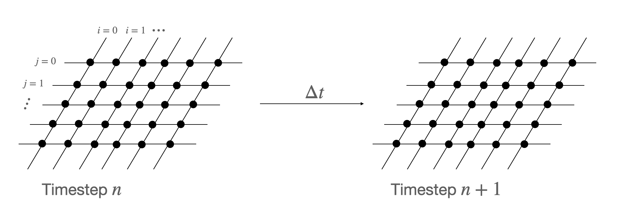
Discretizing
A wave equation relates time derivatives to spatial derivatives. The continuous form for the 2D wave equation is given below. In this equation, $c$ is the speed of sound in the medium, $\eta$ is the viscosity coefficient, and $u$ is the out-of-plane amplitude of the node.
\begin{align} \frac{1}{c^2} \frac{\partial^2{u}}{\partial{t}^2} = \frac{\partial^2{u}}{\partial{x^2}} + \frac{\partial^2{u}}{\partial{y^2}} - \eta \frac{\partial{u}}{\partial{t}} \end{align}In order to discretize this equation, recall the definition of a derivative and its difference approximation:
\begin{align} \frac{d}{dt}u(t) &= \lim_{\Delta t \rightarrow 0} \frac{u(t + \Delta t) - u(t)}{\Delta t}\\ &\approx \frac{u(t + \Delta t) - u(t)}{\Delta t} \end{align}And recall the difference approximation for a second derivative:
\begin{align} \frac{d^2}{dt^2} u(t) &= \frac{ \frac{u(t + \Delta t) - u(t)}{\Delta t} - \frac{u(t) - u(t - \Delta t)}{\Delta t}}{\Delta t}\\ &= \frac{u(t + \Delta t) - 2 u(t) + u(t - \Delta t)}{\Delta t^2} \end{align}Let us introduce a little notation for tidiness
Using the notation introduce above, we can rewrite the difference approximation for the second derivative a bit more concisely:
\begin{align} \frac{d^2}{dt^2}u(t) &= \frac{u_{i,j}^{n+1} - 2u_{i,j}^n + u_{i,j}^{n-1}}{\Delta t^2} \end{align}The same difference approximation can be applied to spatial derivatives. Substituting into the continuous wave equation yields the following difference approximation for the 2D wave equation:
\begin{align} \frac{1}{c^2}\left[\frac{u_{i,j}^{n+1} - 2u_{i,j}^n + u_{i,j}^{n-1}}{\Delta t^2}\right] &= \frac{u_{i+1,j}^n - 2u_{i,j}^n + u_{i-1,j}^n}{\Delta x^2} + \frac{u_{i,j+1}^n - 2u_{i,j}^n + u_{i,j-1}^n}{\Delta y^2} - \eta\left(\frac{u_{i,j}^{n+1} - u_{i,j}^{n-1}}{2\Delta t}\right) \end{align}We're going to solve this equation for $u_{i,j}^{n+1}$. But let's first define a parameter. This parameter is a normalized speed of sound in the medium. For the system to be stable (satisfy the Courant-Friedrichs-Lewy condition it must be less than 0.5.
\begin{align} \rho = \left(\frac{c \Delta t}{\Delta x}\right)^2 < 0.5 \end{align}With this parameter defined, we can solve the above equation for the updated $n+1$ node:
\begin{align} u_{i,j}^{n+1} &= \left[1 + \frac{\eta \Delta t}{2}\right]^{-1}\left\{ \rho\left[ u_{i+1,j}^n + u_{i-1,j}^n + u_{i,j-1}^n + u_{i,j+1}^n - 4u_{i,j}^n\right] + 2u_{i,j}^n - \left[1 - \frac{\eta \Delta t}{2}\right]u_{i,j}^{n-1}\right\} \end{align}Pitch Glide
In a real drum, the speed of sound through the drum is nonlinearly related to the tension in the membrane. We can make the simulation more realistic by calculating $\rho$ each time the drum is updated using the following equation:
\begin{align} \rho_{eff} = \text{min}\left(0.49, \rho_0 +[u_{i,j} \cdot G_{tension}]^2\right) \end{align}Simplification
In the case that $\frac{\eta \Delta t}{2}$ is small, then the first term in the discretized form of the 2D wave equation can be approximated by the first-order Taylor expansion.
\begin{align} \left[1 + \frac{\eta \Delta t}{2}\right]^{-1} \approx \left[1 - \frac{\eta \Delta t}{2}\right] \end{align}This yields the following simplified version of the disretized equation:
\begin{align} u_{i,j}^{n+1} &= \left[1 - \frac{\eta \Delta t}{2}\right]\left\{ \rho\left[ u_{i+1,j}^n + u_{i-1,j}^n + u_{i,j-1}^n + u_{i,j+1}^n - 4u_{i,j}^n\right] + 2u_{i,j}^n - \left[1 - \frac{\eta \Delta t}{2}\right]u_{i,j}^{n-1}\right\} \end{align}Simulation
Clicking "show code" at the top of thiw webpage will reveal two Python simulations below. The first is for 100x100 drum without a nonlinear $\rho$. The amplitude of the center node for the drum is plotted above the power spectrum. The theoretical locations for the drum modes are overlayed on the power spectrum.
The second simulation uses a nonlinear (and exaggerated) rho for a very audible pitch glide.
from IPython.display import Audio
import numpy
import matplotlib.pyplot as plt
from IPython.display import HTML
plt.rcParams["figure.figsize"] = (20,3)
%matplotlib inline

# Initializize drum
n = 100 ;
u = numpy.zeros((n,n));
u1 = numpy.zeros((n,n));
u2 = numpy.zeros((n,n));
uHit = numpy.zeros((n,n));

# Set rho, sample rate, and simulation time
rho = 0.25;
rho_eff = 0.25;
Fs = 48000 ;
time = numpy.arange(0, 1, (1./Fs))

# Array in which to store audio samples
aud = numpy.zeros(len(time)) ;

# Compute middle nodes
x_mid = int(n/2.);
y_mid = int(n/2.);

# Initialize drum amplitudes to a pyramid
for i in range(1, n-1):
    for j in range(1,n-1):
        uHit[i,j] = max(0, 30-(abs(x_mid - i) + abs(y_mid - j)))/30.;

# Zero boundary conditions
uHit[0,:] = 0
uHit[n-1,:] = 0
uHit[:,0] = 0
uHit[:,n-1] = 0

# Indexing variable
tindex = 0;

# Loop through time array
for t in time:

    u = numpy.zeros((n,n))

    # Hit the drum at t=0
    if (t==0):
        u1 = u1 + uHit;

    # Compute updated drum amplitudes
    u[1:n-2,1:n-2] = (1./(1+.0001)) * (rho_eff * (u1[2:n-1,1:n-2]+
                                      u1[0:n-3,1:n-2]+
                                      u1[1:n-2,2:n-1]+
                                      u1[1:n-2,0:n-3]-
                                      4*u1[1:n-2,1:n-2])
                               + 2*u1[1:n-2,1:n-2]
                               - (1-.0001) * (u2[1:n-2,1:n-2]) ) ;

    # Amplitude of center node goes into audio array
    aud[tindex] = u[n//2,n//2] ;

    # Update/store drum state
    u2 = u1;
    u1 = u;

    # Update rho
#     rho_eff = min(0.49, rho + ((1./16)*u[n//2,n//2])**2.)

    # Iterate
    tindex = tindex + 1;


# Plot the center node amplitudes
plt.rcParams["figure.figsize"] = (20,3)
plt.plot(time, aud)
plt.xlabel('time (sec)')
plt.ylabel('amplitude')
plt.title('Center-Node Amplitude and Power Spectrum for 100x100 drum', fontsize=18)
plt.figsize=(20,3)
plt.show()

# Plot the power spectrum
plt.rcParams["figure.figsize"] = (20,3)
Pxxt, freqst = plt.psd(aud,
                     NFFT=len(aud),
                     Fs=48000,
                     window=numpy.hamming(len(aud)),
                     noverlap=50, label='100x100')

# Plot the theoretical mode locations
fundamental = 173
yvals = numpy.linspace(-60, 70)
modes = [1.58, 2.0, 2.24, 2.55, 2.92, 3.0, 3.16, 3.54]
plt.plot(numpy.ones(len(yvals))*fundamental,
             yvals,
             'red',
             alpha=0.5, label='theoretical mode locations')
for i in modes:
    plt.plot(numpy.ones(len(yvals))*fundamental*i,
             yvals,
             'red',
             alpha=0.5)

# Configure plots
plt.xlim([0,1000])
plt.xticks(size=18)
plt.legend(loc='best')
plt.show()

# Output audio
print("Audio - Python synthesized, constant value for rho, 100x100 drum")
Audio(aud, rate=48000)


# Initializize drum
n = 100 ;
u = numpy.zeros((n,n));
u1 = numpy.zeros((n,n));
u2 = numpy.zeros((n,n));
uHit = numpy.zeros((n,n));

# Set rho, sample rate, and simulation time
rho = 0.25;
rho_eff = 0.25;
Fs = 48000 ;
time = numpy.arange(0, 1, (1./Fs))

# Array in which to store audio samples
aud = numpy.zeros(len(time)) ;

# Compute middle nodes
x_mid = int(n/2.);
y_mid = int(n/2.);

# Initialize drum amplitudes to a pyramid
for i in range(1, n-1):
    for j in range(1,n-1):
        uHit[i,j] = max(0, 30-(abs(x_mid - i) + abs(y_mid - j)))/30.;

# Zero boundary conditions
uHit[0,:] = 0
uHit[n-1,:] = 0
uHit[:,0] = 0
uHit[:,n-1] = 0

# Indexing variable
tindex = 0;

# Loop through time array
for t in time:

    u = numpy.zeros((n,n))

    # Hit the drum at t=0
    if (t==0):
        u1 = u1 + uHit;

    # Compute updated drum amplitudes
    u[1:n-2,1:n-2] = (1./(1+.0001)) * (rho_eff * (u1[2:n-1,1:n-2]+
                                      u1[0:n-3,1:n-2]+
                                      u1[1:n-2,2:n-1]+
                                      u1[1:n-2,0:n-3]-
                                      4*u1[1:n-2,1:n-2])
                               + 2*u1[1:n-2,1:n-2]
                               - (1-.0001) * (u2[1:n-2,1:n-2]) ) ;

    # Amplitude of center node goes into audio array
    aud[tindex] = u[n//2,n//2] ;

    # Update/store drum state
    u2 = u1;
    u1 = u;

    # Update rho
    rho_eff = min(0.49, rho + ((1./16)*u[n//2,n//2])**2.)

    # Iterate
    tindex = tindex + 1;


# Plot the center node amplitudes
plt.rcParams["figure.figsize"] = (20,3)
plt.plot(time, aud)
plt.xlabel('time (sec)')
plt.ylabel('amplitude')
plt.title('Center-Node Amplitude and Power Spectrum for 100x100 drum - nonlinear rho', fontsize=18)
plt.figsize=(20,3)
plt.show()

# Plot the power spectrum
plt.rcParams["figure.figsize"] = (20,3)
Pxxt, freqst = plt.psd(aud,
                     NFFT=len(aud),
                     Fs=48000,
                     window=numpy.hamming(len(aud)),
                     noverlap=50, label='100x100')

# Plot the theoretical mode locations
fundamental = 173
yvals = numpy.linspace(-60, 70)
modes = [1.58, 2.0, 2.24, 2.55, 2.92, 3.0, 3.16, 3.54]
plt.plot(numpy.ones(len(yvals))*fundamental,
             yvals,
             'red',
             alpha=0.5, label='theoretical mode locations')
for i in modes:
    plt.plot(numpy.ones(len(yvals))*fundamental*i,
             yvals,
             'red',
             alpha=0.5)

# Configure plots
plt.xlim([0,1000])
plt.xticks(size=18)
plt.legend(loc='best')
plt.show()

# Output audio
print("Audio - Python synthesized, nonlinear rho, 100x100 drum")
Audio(aud, rate=48000)


# Initializize drum
n = 100 ;
u = numpy.zeros((n,n));
u1 = numpy.zeros((n,n));
u2 = numpy.zeros((n,n));
uHit = numpy.zeros((n,n));

# Set rho, sample rate, and simulation time
# rho = 0.4;
rho_eff = 0.25;
Fs = 48000 ;
time = numpy.arange(0, 1, (1./Fs))

# Array in which to store audio samples
aud = numpy.zeros(len(time)) ;

# Compute middle nodes
x_mid = int(n/2.);
y_mid = int(n/2.);

# Initialize drum amplitudes to a pyramid
for i in range(1, n-1):
    for j in range(1,n-1):
        uHit[i,j] = max(0, 30-(abs(x_mid - i) + abs(y_mid - j)))/30.;

# Zero boundary conditions
uHit[0,:] = 0
uHit[n-1,:] = 0
uHit[:,0] = 0
uHit[:,n-1] = 0

# Indexing variable
tindex = 0;

# Loop through time array
for t in time:

    u = numpy.zeros((n,n))

    # Hit the drum at t=0
    if (t==0):
        u1 = u1 + uHit;

    # Compute updated drum amplitudes
    u[1:n-2,1:n-2] = ((1-.0001)) * (rho_eff * (u1[2:n-1,1:n-2]+
                                      u1[0:n-3,1:n-2]+
                                      u1[1:n-2,2:n-1]+
                                      u1[1:n-2,0:n-3]-
                                      4*u1[1:n-2,1:n-2])
                               + 2*u1[1:n-2,1:n-2]
                               - (1-.0001) * (u2[1:n-2,1:n-2]) ) ;

    # Amplitude of center node goes into audio array
    aud[tindex] = u[n//2,n//2] ;

    # Update/store drum state
    u2 = u1;
    u1 = u;

    # Update rho
#     rho_eff = min(0.49, rho + ((1./16)*u[n//2,n//2])**2.)

    # Iterate
    tindex = tindex + 1;


# Plot the center node amplitudes
plt.rcParams["figure.figsize"] = (20,3)
plt.plot(time, aud)
plt.xlabel('time (sec)')
plt.ylabel('amplitude')
plt.title('Center-Node Amplitude and Power Spectrum for 100x100 drum - Taylor approximation', fontsize=18)
plt.figsize=(20,3)
plt.show()

# Plot the power spectrum
plt.rcParams["figure.figsize"] = (20,3)
Pxxt, freqst = plt.psd(aud,
                     NFFT=len(aud),
                     Fs=48000,
                     window=numpy.hamming(len(aud)),
                     noverlap=50, label='100x100')

# Plot the theoretical mode locations
fundamental = 173
yvals = numpy.linspace(-60, 70)
modes = [1.58, 2.0, 2.24, 2.55, 2.92, 3.0, 3.16, 3.54]
plt.plot(numpy.ones(len(yvals))*fundamental,
             yvals,
             'red',
             alpha=0.5, label='theoretical mode locations')
for i in modes:
    plt.plot(numpy.ones(len(yvals))*fundamental*i,
             yvals,
             'red',
             alpha=0.5)

# Configure plots
plt.xlim([0,1000])
plt.xticks(size=18)
plt.legend(loc='best')
plt.show()

# Output audio
print("Audio - Python synthesized, constant value for rho, 100x100 drum - Taylor approximation")
Audio(aud, rate=48000)

