Tree Ring Steganography
V. Hunter Adams
import numpy
import matplotlib.pyplot as plt
from IPython.core.display import HTML
from matplotlib import animation, rc
import matplotlib
from IPython.display import HTML
from IPython.display import Audio
from IPython.display import clear_output
from struct import pack
import wave
from matplotlib.pyplot import figure
from scipy.io import wavfile
HTML('''<script>
code_show=true;
function code_toggle() {
if (code_show){
$('div.input').hide();
} else {
$('div.input').show();
}
code_show = !code_show
}
$( document ).ready(code_toggle);
</script>
<form action="javascript:code_toggle()"><input type="submit" value="Click here to toggle on/off the raw code."></form>''')
Patterns in nature
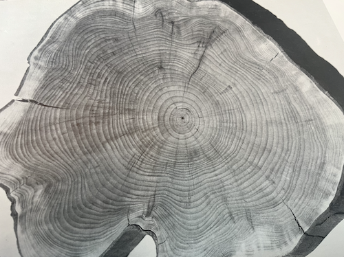
Patterns decorate nearly every corner of nature. Many of these patterns possess an "order" which gives them a distinct aesthetic. Tree rings look like tree rings, snowflakes look like snowflakes, etc. But there's also a randomness in each of these patterns that allow for many variations on a theme. So long as we maintain the order which gives a particular pattern its recognizable form, we can hide information in the randomness. Tree rings offer an interesting proof-of-concept for this idea.
Order and randomness in tree rings
Tree rings have certain properties which make them look like tree rings. Obviously, each ring must form a closed curve. Furthermore, if you consider the rings from the inside out, each must fully circumscribe all previous rings, and the rings must not cross themselves or the rings they circumscribe.
But not all the rings are exactly the same shape. Variations in growing conditions lead to variations in ring shape, and we can hide information in these variations. These variations must also adhere to certain rules in order to "look right." They can't be too high-frequency, and there can't be too much deviation in the fundamental shape of the tree from ring to ring. But even under these constraints, the total space of natural-looking ring shapes is quite large!
How do you build a tree ring?
Because the tree ring is a closed curve, we can construct it with linear combinations of sine and cosine functions.
\begin{align} x(\theta) &= \sum_{i=1}^{10} A_i \cos{i \theta} && \theta\in[0,2\pi]\\ y(\theta) &= \sum_{i=1}^{10} B_i \sin{i \theta} && \theta\in[0,2\pi] \end{align}In principle, the above sum could include the $i=0$ term, but we'll just suppose that our origin is at the center of the ring so that there's no DC offset. The first term in the above summations ($i=1$) constructs a circle, and the subsequent terms add increasingly-high-frequency wiggles to that circle. We'll use these wiggles to hide information. The summation only goes to 10 because that's all we need to encode ASCII, though it could include higher frequencies.
Encoding
We can encode a message in the summation coefficients $A_i$ and $B_i$. Let's expand these summations:
\begin{align} x(\theta) &= A_1\cos{\theta} + A_2\cos{2\theta} + A_3\cos{3\theta} + A_4\cos{4\theta} + A_5\cos{5\theta} + A_6\cos{6\theta} + A_7\cos{7\theta} + A_8\cos{8\theta} + A_9\cos{9\theta} + A_{10}\cos{10\theta}\\ y(\theta) &= B_1\sin{\theta} + B_2\sin{2\theta} + B_3\sin{3\theta} + B_4\sin{4\theta} + B_5\sin{5\theta} + B_6\sin{6\theta} + B_7\sin{7\theta} + B_8\sin{8\theta} + B_9\sin{9\theta} + B_{10}\sin{10\theta} \end{align}As mentioned previously, the first terms ($A_1$ and $B_1$) just set the size of the ring. This won't encode any information, it will instead enforce some of the "order" which makes tree rings look like tree rings. These provide a mechanism for making certain that our rings don't cross, and that each completely contains all which precede it.
Experimentation shows that the rings look most "natural" if $A_2$ and $B_2$ are zero, so these too won't encode any information. But we can put information on $A_{3\longrightarrow 10}$! One straightforward way to do this is to assign each of these 8 coefficients using the 8 bits from an ASCII character. Let's suppose, for instance, that we want to encode "Hi" in a tree ring by putting "H" on the trajectory of x coordinates and "i" on the trajetory of y coordinates. Let's consider the ASCII representations of these two characters:
\begin{align} \text{H} &\longrightarrow 01001000\\ \text{i} &\longrightarrow 01101001 \end{align}These 1's and 0's set our coefficients. Let's suppose that we set $A_1$ and $B_1$ to 10, if we keep our higher-amplitude "wiggles" at an amplitude of about 1, things look very natural. So, our trajectory of x and y coordinates, with "H" encoded into the former and "i" encoded into the latter, becomes:
\begin{align} x(\theta) &= 10\cos{\theta} + 0\cos{2\theta} + 0\cos{3\theta} + 1\cos{4\theta} + 0\cos{5\theta} + 0\cos{6\theta} + 1\cos{7\theta} + 0\cos{8\theta} + 0\cos{9\theta} + 0\cos{10\theta}\\ y(\theta) &= 10\sin{\theta} + 0\sin{2\theta} + 0\sin{3\theta} + 1\sin{4\theta} + 1\sin{5\theta} + 0\sin{6\theta} + 1\sin{7\theta} + 0\sin{8\theta} + 0\sin{9\theta} + 1\sin{10\theta} \end{align}Note that $A_1$ and $B_1$ are 10 (which just sets the size of the ring), $A_2$ and $B_2$ are zero (just looks nice), and $A_{3\longrightarrow 10}$ are set according to each bit in the ASCII representations for "H" and "i". We could plot the x and y coordinates separately, and we'd get the two plots shown below.
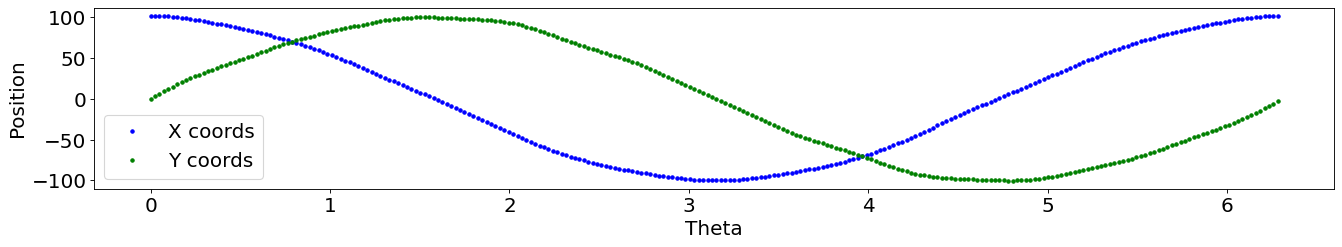
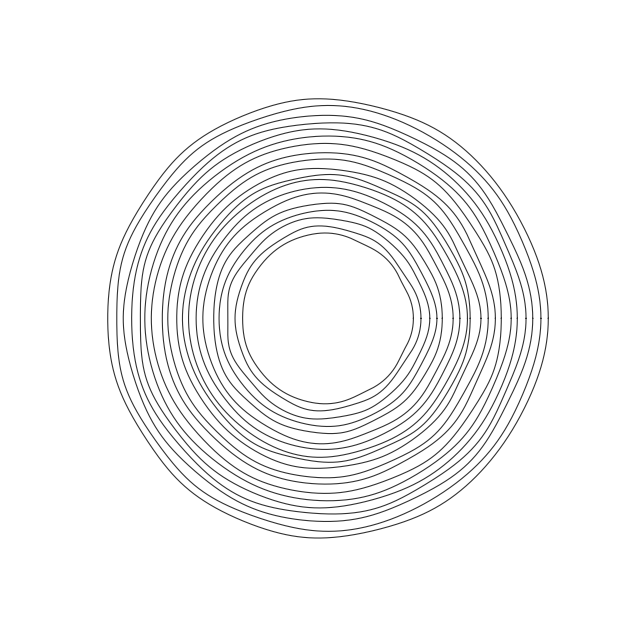
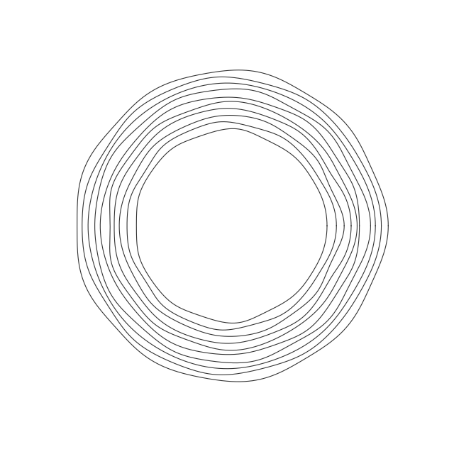
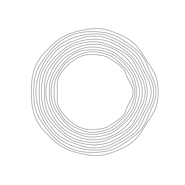
But if we use each pair of x and y coordinates to specify a coordinate in 3D space, the sequence of coordinates generates a closed shape that looks an awful lot like a tree-ring.

We can use this strategy to encode all sorts of messages. Every time we want to add two more characters to our message, we just increase the values of $A_1$ and $B_1$ a bit and make another ring.
Decoding
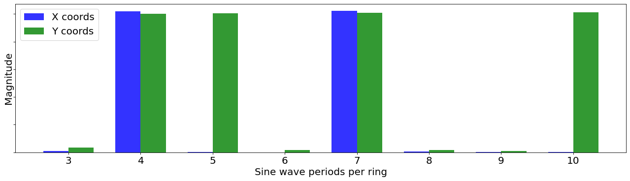
Having generated a shape which encodes our message, how do we extract the message from the shape? Sample it, perform an FFT, and check for the existence or non-existence of power at each of the frequencies of relevance. Sampling the above curve 2048 times, performing an FFT, and computing the power spectrum at the frequencies of interest yields the plot below, from which we can easily extract the ASCII bits associated with the x and y coordinates.
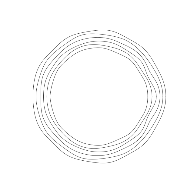
These decoding process becomes particularly clear if, instead of nesting the tree rings, we instead smoothly morph each into the next. This allows for us to observe the frequency content of the rings change from that associated with one character to that associated with the next.
def synthesis(an, bn, cn, dn):
theta = numpy.linspace(0, 2*numpy.pi, 2048)
inner_sum_x = numpy.zeros(len(theta))
inner_sum_y = numpy.zeros(len(theta))
for i in range(len(an)):
first_x = an[i]*numpy.cos((i+1)*theta)
second_x = bn[i]*numpy.sin((i+1)*theta)
inner_sum_x += (first_x + second_x)
first_y = cn[i]*numpy.cos((i+1)*theta)
second_y = dn[i]*numpy.sin((i+1)*theta)
inner_sum_y += (first_y + second_y)
return inner_sum_x, inner_sum_y
plaintext = "Cornell Duffield College of Engineering"
figure(figsize=(8, 8), dpi=80)
count = 0 ;
iterator = 100
ans = numpy.zeros(10)
bns = numpy.zeros(11)
cns = numpy.zeros(11)
dns = numpy.zeros(10)
ans_list = []
dns_list = []
count = 0
makered = 0
for i in plaintext:
if (count==0):
ans = numpy.insert(numpy.array([float(i) for i in f"{ord(i):08b}"]), 0, 0)
ans = numpy.insert(ans, 0, iterator)
ans_list.append(ans)
count += 1
elif (count==1):
dns = numpy.insert(numpy.array([float(i) for i in f"{ord(i):08b}"]), 0, 0)
dns = numpy.insert(dns, 0, iterator)
dns_list.append(dns)
count = 0
xvals, yvals = synthesis(ans, bns, cns, dns)
# In case you want to color a particular ring
if (makered==55):
tempx = xvals[0::8]
tempy = yvals[0::8]
plt.plot(tempx, tempy,'r.',
alpha=0.8, lw=0.001, markersize=2)
for j in range(len(xvals[0::8])):
plt.plot([0, tempx[j]], [0, tempy[j]], 'b-', lw=0.5, alpha=0.5)
plt.plot(0, 0, 'r*')
makered += 1
else:
plt.plot(xvals, yvals,
alpha=0.8, color='black', lw=1)
makered += 1
iterator += 6 + numpy.random.uniform(0, 5)
ans_list.append(ans_list[0])
dns_list.append(dns_list[0])
plt.axis('off')
plt.axis('scaled')
plt.savefig("Cornell_Duffield.png")
plt.show()
figure(figsize=(20, 3), dpi=80)
plt.plot(numpy.linspace(0, 2*numpy.pi, 256), xvals[0::8], 'b.')
plt.plot(numpy.linspace(0, 2*numpy.pi, 256), yvals[0::8], 'g.')
plt.legend(['X coords', 'Y coords'], fontsize=18)
plt.ylabel('Position', fontsize=18)
plt.xlabel('Theta', fontsize=18)
plt.xticks(fontsize=18)
plt.yticks(fontsize=18)
plt.savefig('timedomain.png', bbox_inches='tight')
plt.show()
figure(figsize=(20, 3), dpi=80)
plt.plot(numpy.arange(3, 11)+0.05, [numpy.abs(i) for i in numpy.fft.fft(xvals)][3:11], 'b*')
plt.plot(numpy.arange(3, 11)-0.05, [numpy.abs(i) for i in numpy.fft.fft(yvals)][3:11], 'g*')
plt.xticks(fontsize=18)
plt.yticks(fontsize=18, visible=False)
# plt.legend(['Frequency content of X coords', 'Frequency content of Y coords'], fontsize=18)
plt.ylabel('Magnitude', fontsize=18)
plt.xlabel('Sine wave periods per ring', fontsize=18)
plt.savefig('FFT.png', bbox_inches='tight')
plt.show()
fig, ax = plt.subplots(figsize=(20, 5), dpi=80)
# compute FFT magnitudes once
fft_x = numpy.abs(numpy.fft.fft(xvals))[3:11]
fft_y = numpy.abs(numpy.fft.fft(yvals))[3:11]
# x positions (frequency bins)
idx = numpy.arange(3, 11)
# bar width
w = 0.35
# side-by-side bars
ax.bar(idx - w/2, fft_x, width=w, color='b', label='X coords', alpha=0.8)
ax.bar(idx + w/2, fft_y, width=w, color='g', label='Y coords', alpha=0.8)
ax.set_xticks(idx)
ax.tick_params(axis='x', labelsize=18)
ax.tick_params(axis='y', labelsize=18)
ax.tick_params(axis='y', labelleft=False)
ax.set_ylabel('Magnitude', fontsize=18)
ax.set_xlabel('Sine wave periods per ring', fontsize=18)
ax.legend(fontsize=18)
# ax.legend(fontsize=18)
plt.savefig('FFT.png', bbox_inches='tight')
plt.show()
# fig1 = plt.figure(figsize=(7, 7))
fig1, axis1 = plt.subplots(1,2, figsize=(20, 9))
axis1[0].set_xlim([-130, 130])
axis1[0].set_ylim([-130, 130])
axis1[0].set_title("Encoding messages in tree rings", fontsize=24)
bigxlist = []
bigylist = []
ann = axis1[0].annotate(plaintext[0:2], xy=(-130, 110), xytext=(-130, 110), fontsize=14, alpha=0.8)
axis1[0].axis('off')
axis1[1].set_xlim([2, 11])
axis1[1].set_ylim([-100, 1100])
axis1[1].annotate("binary slice threshold", xy=(8.5, 505), xytext=(8.5, 505), fontsize=12, alpha=0.4)
transition_frames=6
axis1[1].set_xlabel('Sine wave periods per ring\n(Each represents a bit in an ASCII character)', fontsize=18)
axis1[1].set_ylabel('Magnitude', fontsize=18)
axis1[1].set_yticklabels([])
axis1[1].set_xticklabels(['',3,4,5,6,7,8,9,10,''],fontsize=18)
axis1[1].plot(numpy.arange(2,12), numpy.ones(10)*500, 'black', alpha=0.4)
lines, = axis1[0].plot([], [], lw = 6)
# lines1, = axis1[1].plot([], [], 'b*', markersize=20, label='x coord frequency content')
# lines2, = axis1[1].plot([], [], 'g*', markersize=20, label='y coord frequency content')
xpos = numpy.arange(3, 11)
lines1 = axis1[1].bar(
xpos + 0.15,
numpy.zeros(8),
width=0.25,
alpha=0.7,
label='x coord frequency content'
)
lines2 = axis1[1].bar(
xpos - 0.15,
numpy.zeros(8),
width=0.25,
alpha=0.7,
label='y coord frequency content'
)
axis1[1].legend(bbox_to_anchor=(0, 1.08), loc='upper left', fontsize=12, ncol=2)
last_frame = 0
# what will our line dataset
# contain?
def init1():
lines.set_data([], [])
for bar in lines1:
bar.set_height(0)
for bar in lines2:
bar.set_height(0)
return (lines, *lines1, *lines2)
# initializing empty values
# for x and y co-ordinates
xdata1, ydata1 = [], []
# animation function
def animates(i):
frame = i//transition_frames
if (frame != last_frame):
ann.set_text(plaintext[0:(frame+1)*2])
lastx, lasty = synthesis(ans_list[frame], numpy.zeros(11), numpy.zeros(11), dns_list[frame])
comingx, comingy = synthesis(ans_list[frame+1], numpy.zeros(11), numpy.zeros(11), dns_list[frame+1])
weight = (i%transition_frames)/(1.0*transition_frames)
newx = (1-weight)*lastx + weight*comingx
newy = (1-weight)*lasty + weight*comingy
xfreq = [numpy.abs(k) for k in numpy.fft.fft(newx)][3:11]
yfreq = [numpy.abs(k) for k in numpy.fft.fft(newy)][3:11]
lines.set_data(newx, newy)
global bigxlist
global bigylist
bigxlist.extend(newx)
bigylist.extend(newy)
for bar, h in zip(lines1, xfreq):
bar.set_height(h)
for bar, h in zip(lines2, yfreq):
bar.set_height(h)
# return (lines, lines1, lines2,)
return (lines, *lines1, *lines2)
# calling the animation function
anim1 = animation.FuncAnimation(fig1, animates, init_func = init1,
frames = transition_frames*(len(ans_list)-1), interval = 30, blit = True)
# saves the animation in our desktop
anim1.save('wigglerings.mp4', writer = 'ffmpeg', fps = 30)
rc('animation', html='jshtml')
plt.close()
anim1