import numpy
import matplotlib.pyplot as plt
from IPython.display import Audio
from IPython.display import Image
from scipy import signal
from scipy.fft import fftshift
from scipy.io import wavfile
plt.rcParams['figure.figsize'] = [12, 4]
from IPython.core.display import HTML
HTML("""
<style>
.output_png {
    display: table-cell;
    text-align: center;
    vertical-align: middle;
}
</style>
""")
Page contents
Before you start
- This document is a supplement for the birdsong synthesis lab assignment for ECE 4760.
- Please read the Direct Digital Synthesis page before reading this page.
- Please note: This webpage uses Python to generate a song and then play it back. In class, you will both compute and synthesize the song in realtime.
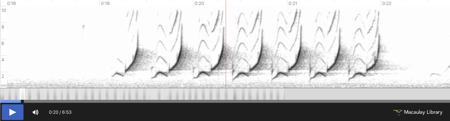
Deconstructing the song
The song of a northern cardinal can be decomposed into three sound primitives: a low-frequency swoop at the beginning of each call, a chirp after each swoop which moves rapidly from low frequency to high frequency, and silence which separates each swoop/chirp combination. We will synthesize each of these primitives separately, and then compose them to reconstruct the song.
Swoop
Swoop Analysis
By pasting the above spectrogram in Keynote or PowerPoint and drawing lines on it, you can determine that the length of the chirp is approximately 130 ms. Since the DAC gathers audio samples at 40kHz, this means that the chirp lasts for $0.130\text{sec} \cdot \frac{40000\text{ samples}}{1\text{ sec}} = 5200\text{ samples}$. We'll approximate the frequency curve by sine wave of the form:
\begin{align} y = k\sin{mx} + b \end{align}where $y$ is the frequency in Hz, and $x$ is the number of audio samples since the chirp began. Since the swoop starts and ends at 1.74kHz and peaks at 2kHz, we can setup the following system of equations to solve for the unknown parameters $k$, $b$, and $m$:
\begin{align} 1740 &= k\sin{m\cdot 0} + b\\ 1740 &= k\sin{m\cdot 5200} + b\\ 2000 &= k\sin{m\cdot 2600} + b \end{align}From which we can find $b=1740$, $k = -260$, $m = \frac{-\pi}{5200}$. So, the equation is given by:
\begin{align} y = -260 \sin{\left(-\frac{\pi}{5200} \cdot x\right)} + 1740 \end{align}Plot the simulated swoop of frequencies:
plt.plot(-260*numpy.sin(-numpy.pi/5200*numpy.arange(5200)) + 1740)
plt.xlabel('Audio samples'); plt.ylabel('Hz'); plt.title('Swoop frequencies')
plt.show()

Swoop Simulation
Some DDS parameters, including the sample rate (44kHz), a 256-entry sine table, and the constant $2^{32}$:
Fs = 40000 #audio sample rate
sintable = numpy.sin(numpy.linspace(0, 2*numpy.pi, 256))# sine table for DDS
two32 = 2**32 #2^32
And now we can synthesize audio samples.
swoop = list(numpy.zeros(5200)) # a 5200-length array (130ms @ 44kHz) that will hold swoop audio samples
DDS_phase = 0 # current phase
for i in range(len(swoop)):
    frequency = -260.*numpy.sin((-numpy.pi/5200)*i) + 1740 # calculate frequency
    DDS_increment = frequency*two32/Fs # update DDS increment
    DDS_phase += DDS_increment # update DDS phase by increment
    DDS_phase = DDS_phase % (two32 - 1) # need to simulate overflow in python, not necessary in C
    swoop[i] = sintable[int(DDS_phase/(2**24))] # can just shift in C
In order to avoid non-natural clicks, we must ramp the amplitude smoothly from 0 to its max amplitude, and then ramp it down. We'll do this by multiplying the chirp by the linear ramp function shown below:
# Amplitude modulate with a linear envelope to avoid clicks
amplitudes = list(numpy.ones(len(swoop)))
amplitudes[0:1000] = list(numpy.linspace(0,1,len(amplitudes[0:1000])))
amplitudes[-1000:] = list(numpy.linspace(0,1,len(amplitudes[-1000:]))[::-1])
amplitudes = numpy.array(amplitudes)
plt.plot(amplitudes);plt.title('Amplitude envelope');plt.show()

# Finish with the swoop
swoop = swoop*amplitudes

Here is what the swoop looks like:
plt.plot(swoop);plt.title('Amplitude-modulated swoop');plt.show()

And here is what it sounds like:
Audio(swoop, rate=40000)
Chirp
Chirp Analysis
By pasting the above spectrogram in Keynote and drawing lines on it, you can determine that the length of the chirp is also approximately 130 ms (5720 samples). We'll approximate the frequency curve by a quadratic equation of the form:
\begin{align} y = kx^2 + b \end{align}where $y$ is the frequency in Hz, and $x$ is the number of audio samples since the chirp began. Since the chirp starts at 2kHz and ends at 7kHz, we can setup the following system of equations to solve for the unknown parameters $k$ and $b$:
\begin{align} 2000 &= k(0^2) + b\\ 7000&= k(5200^2) + b \end{align}This is two equations with two unknowns. Solving, we find that $b=2000$ and $k\approx 1.53 \times 10^{-4}$. So the quadratic equation for the chirp is:
\begin{align} y &= \left(1.84\times 10^{-4}\right)x^2 + 2000 && \text{for $x\in[0, 5200]$} \end{align}Plot the simulated chirp frequency sweep:
plt.plot(1.84e-4 * numpy.arange(5200)**2. + 2000);plt.title('Chirp frequencies');plt.show()

Chirp Simulation
And now we can synthesize audio samples.
chirp = list(numpy.zeros(5200)) # a 5720-length array (130ms @ 44kHz) that will hold chirp audio samples
DDS_phase = 0 # current phase
for i in range(len(chirp)):
    frequency = (1.84e-4)*(i**2.) + 2000 # update DDS frequency
    DDS_increment = frequency*two32/Fs # update DDS increment
    DDS_phase += DDS_increment # update DDS phase
    DDS_phase = DDS_phase % (two32 - 1) # need to simulate overflow in python, not necessary in C
    chirp[i] = sintable[int(DDS_phase/(2**24))] # can just shift in C
In order to avoid non-natural clicks, we must ramp the amplitude smoothly from 0 to its max amplitude, and then ramp it down. We'll do this by multiplying the chirp by the linear ramp function shown below:
# Amplitude modulate with a linear envelope to avoid clicks
amplitudes = list(numpy.ones(len(chirp)))
amplitudes[0:1000] = list(numpy.linspace(0,1,len(amplitudes[0:1000])))
amplitudes[-1000:] = list(numpy.linspace(0,1,len(amplitudes[-1000:]))[::-1])
amplitudes = numpy.array(amplitudes)

# Finish with the chirp
chirp = chirp*amplitudes
The entire amplitude-modulated chirp looks like this:
plt.plot(chirp);plt.title('Amplitude-modulated chirp');plt.show()

And it sounds like this:
Audio(chirp, rate=40000)
silence = numpy.zeros(5200)
song = []
for i in range(5):
    song.extend(list(swoop))
    song.extend(list(chirp))
    song.extend(list(silence))
song.extend(list(swoop))
song.extend(list(chirp))
song.extend(list(silence))
song = numpy.array(song)

plt.plot(song);plt.title('Full song');plt.show()

Listen to it:
Audio(song, rate=40000)
And view the spectrogram of the Python-generated song:
f, t, Sxx = signal.spectrogram(song, Fs)
plt.pcolormesh(t, f, Sxx,  shading='gouraud')
plt.ylabel('Hz'); plt.xlabel('Time (sec)')
plt.title('Spectrogram of Python-generated birdsong')
plt.ylim([0,10000])
plt.show()
