Picasso, by way of Fourier

Using Fourier series to draw, animate, and sonify Picasso's line drawings

V. Hunter Adams

HTML('''<script>
code_show=true; 
function code_toggle() {
 if (code_show){
 $('div.input').hide();
 } else {
 $('div.input').show();
 }
 code_show = !code_show
} 
$( document ).ready(code_toggle);
</script>
<form action="javascript:code_toggle()"><input type="submit" value="Click here to toggle on/off the raw code."></form>''')

---

• Introduction
• Mathematical background

  • Remember Fourier Series?
  • Fourier Series for a polyline curve
  • 2D curves in space are two polyline curves
  • Re-parametrizing from time to distance along curve

• Encoding
• Visualizations and sonifications

  • Abstraction
  • Morphing
  • Sonification

---

import numpy
import matplotlib.pyplot as plt
from IPython.core.display import HTML
from matplotlib import animation, rc
import matplotlib
from IPython.display import HTML
from IPython.display import Audio
from IPython.display import clear_output
from struct import pack
import wave
from scipy.io import wavfile

Introduction

I really like Picasso's studies of abstraction, in which he reduces a complex subject to its simplest representation which retains recognizability. The Bull is probably the most famous example, but all of his line drawings are interesting studies of abstraction.

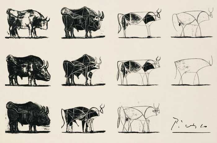
This document uses Fourier Series to recreate some of Picasso's line drawings, to morph one drawing into another, and to sonify the drawings (i.e., to create a sound which carries the same information as the line drawing). This sound can be used to generate Picasso's images on an oscilloscope.

The Fourier Series provides a systematic, quantifiable method for studying abstraction, and for finding the level of complexity that is required to make a particular subject recognizable. It's not a perfect tool for doing so. The Fourier Series can only generate closed shapes, and it adds complexity by adding higher-frequency content to that closed shape. So, all forms "simplify" ultimately into circles or ellipses.

Move the slider below. How many Fourier coefficients does it take for the abstraction to become something recognizable?

anim1

Once Loop Reflect

---

Mathematical background

The content in this section comes from An Algebra of Geometric Shapes by Ghosh and Jain and Elliptical Fourier Features of a Closed Contour by Kuhl and Giardina.

Remember Fourier Series?

Recall our old friend the the Fourier Series. For some function $f(t)$ which is periodic over a period of time $T$ (that is, $f(t+nT) = f(t)$ for any integer $n$ and real $t$), then we can express that function as a sum of sines and cosines of various amplitudes. The amplitude of each sine and cosine wave in that sum can be solved for using the function $f(t)$ and the period $T$, as shown below. If you're curious where these expressions come from, please see one of my other webpages on the topic.

\begin{align} f(t) &= a_0 + \sum_{n=0}^{\infty}\left(a_n \cos{\frac{2\pi n t}{T}} + b_n \sin{\frac{2\pi n t}{T}}\right)\\ \\ a_0 &= \frac{1}{T} \int_0^T f(t) dt\\ a_n &= \frac{2}{T} \int_0^T f(t) \cos{\frac{2\pi n t}{T}} dt\\ b_n &= \frac{2}{T} \int_0^T f(t) \sin{\frac{2\pi n t}{T}} dt \end{align}

Fourier Series for a polyline curve

Suppose that the function for which we are generating a Fourier Series is described by a sequence of points connected by lines. One such "polyline curve" is given below.

def demoPiecewise():
    y = numpy.array([5., 10., 3., 14., 3., 2., 4., 5., 1., 5.])
    x = numpy.arange(10)
    plt.figure(figsize=(15,5))
    plt.plot(x, y, 'b.-')
    plt.ylim([-1, 16])
    plt.title('Polyline curve $x(t)$', fontsize=18)
    plt.text(-.1, 4, '$t_{j=0}$', fontsize = 16)
    plt.text(0.9, 10.4, '$t_{j=1}$', fontsize = 16)
    plt.text(1.9, 2, '$t_{j=2}$', fontsize = 16)
    plt.text(2.9, 14.4, '$t_{j=3}$', fontsize = 16)
    plt.text(3.9, 1.9, '$t_{j=4}$', fontsize = 16)
    plt.text(4.9, 1.1, '$t_{j=5}$', fontsize = 16)
    plt.text(5.9, 4.4, '$t_{j=6}$', fontsize = 16)
    plt.text(6.9, 5.4, '$t_{j=7}$', fontsize = 16)
    plt.text(7.9, 0., '$t_{j=8}$', fontsize = 16)
    plt.text(8.9, 5.4, '$t_{j=9}$', fontsize = 16)
    plt.show()
demoPiecewise()

This curve, $x(t)$, can be described by the Fourier Series shown below.

\begin{align} x(t) &= a_0 + \sum_{n=0}^{\infty}\left(a_n \cos{\frac{2\pi n t}{T}} + b_n \sin{\frac{2\pi n t}{T}}\right) \end{align}

We're going to solve for those coefficients, $a_0$, $a_n$, and $b_n$. In order to do so, however, we'll use a little trick! Let us consider the first time derivative for $x(t)$, given by $\dot{x}(t)$. This function can also be represented by a Fourier Series, with a different set of coefficients. Let's call those coefficients $\alpha_n$ and $\beta_n$ (and note that the constant $a_0$ disappears when we take the derivative).

\begin{align} \dot{x}(t) &= \sum_{n=0}^{\infty}\left(\alpha_n \cos{\frac{2\pi n t}{T}} + \beta_n \sin{\frac{2\pi n t}{T}}\right) \end{align}

We can solve for $\alpha_n$ and $\beta_n$, and then we'll use those to solve for $a_n$ and $b_n$. From above, we know that:

\begin{align} \alpha_n &= \frac{2}{T} \int_0^T \dot{x}(t) \cos{\frac{2\pi n t}{T}} dt\\ \beta_n &= \frac{2}{T} \int_0^T \dot{x}(t) \sin{\frac{2\pi n t}{T}} dt \end{align}

The integral over the whole period $T$ is equal to the sum of the integrals over each of the piecewise linear segments . . .

\begin{align} \alpha_n &= \frac{2}{T} \int_0^T \dot{x}(t) \cos{\frac{2\pi n t}{T}} dt\\ &= \frac{2}{T}\left[\sum_{j=1}^K \int_{t_{j-1}}^{t_j} \dot{x}(t) \cos{\frac{2\pi n t}{T}} dt\right]\\ \beta_n &= \frac{2}{T} \int_0^T \dot{x}(t) \sin{\frac{2\pi n t}{T}} dt\\ &= \frac{2}{T}\left[\sum_{j=1}^K \int_{t_{j-1}}^{t_j} \dot{x}(t) \sin{\frac{2\pi n t}{T}} dt\right] \end{align}

But the derivative over each linear segment is just a constant! So this simplifies . . .

\begin{align} \alpha_n &= \frac{2}{T}\left[\sum_{j=1}^K \frac{\Delta x_j}{\Delta t_j} \int_{t_{j-1}}^{t_j} \cos{\frac{2\pi n t}{T}} dt\right]\\ \beta_n &= \frac{2}{T}\left[\sum_{j=1}^K \frac{\Delta x_j}{\Delta t_j} \int_{t_{j-1}}^{t_j} \sin{\frac{2\pi n t}{T}} dt\right] \end{align}

Those final integrals are easy!

\begin{align} \alpha_n &= \frac{2}{T}\sum_{j=1}^K \frac{\Delta x_j}{\Delta t_j} \frac{T}{2\pi n} \left(\sin{\frac{2\pi n t_j}{T}} - \sin{\frac{2\pi n t_{j-1}}{T}} \right)\\ &= \frac{1}{\pi n}\sum_{j=1}^K \frac{\Delta x_j}{\Delta t_j} \left(\sin{\frac{2\pi n t_j}{T}} - \sin{\frac{2\pi n t_{j-1}}{T}} \right)\\ \beta_n &= - \frac{2}{T}\sum_{j=1}^K \frac{\Delta x_j}{\Delta t_j} \frac{T}{2\pi n} \left(\cos{\frac{2\pi n t_j}{T}} - \cos{\frac{2\pi n t_{j-1}}{T}} \right)\\ &= - \frac{1}{\pi n}\sum_{j=1}^K \frac{\Delta x_j}{\Delta t_j} \left(\cos{\frac{2\pi n t_j}{T}} - \cos{\frac{2\pi n t_{j-1}}{T}} \right) \end{align}

We're halfway there. We'll solve for $a_n$ and $b_n$ by coming up with another equation for the Fourier Series of $\dot{x}(t)$ and setting those two equations equal to one another. The second representation for $\dot{x}(t)$ comes from directly differentiating the expression for $x(t)$:

\begin{align} \dot{x}(t) &= \sum_{n=0}^{\infty}\left(- \frac{2\pi n}{T} a_n \sin{\frac{2\pi n t}{T}} + \frac{2 \pi n}{T} b_n \cos{\frac{2\pi n t}{T}}\right) \end{align}

Matching coefficients from the two representations gives:

\begin{align} - \frac{2\pi n}{T} a_n &= - \frac{1}{\pi n}\sum_{j=1}^K \frac{\Delta x_j}{\Delta t_j} \left(\cos{\frac{2\pi n t_j}{T}} - \cos{\frac{2\pi n t_{j-1}}{T}} \right)\\ \frac{2 \pi n}{T} b_n &= \frac{1}{\pi n}\sum_{j=1}^K \frac{\Delta x_j}{\Delta t_j} \left(\sin{\frac{2\pi n t_j}{T}} - \sin{\frac{2\pi n t_{j-1}}{T}} \right) \end{align}

And solving for $a_n$ and $b_n$ . . .

\begin{align} a_n &= \frac{T}{2 \pi^2 n^2}\sum_{j=1}^K \frac{\Delta x_j}{\Delta t_j} \left(\cos{\frac{2\pi n t_j}{T}} - \cos{\frac{2\pi n t_{j-1}}{T}} \right)\\ b_n &= \frac{T}{2 \pi^2 n^2}\sum_{j=1}^K \frac{\Delta x_j}{\Delta t_j} \left(\sin{\frac{2\pi n t_j}{T}} - \sin{\frac{2\pi n t_{j-1}}{T}} \right) \end{align}

We could also solve for the DC component, $a_0$, but for our purposes we actually needn't do so. We'll just have all of our curves centered on the origin, and our DC components will be zero.

2D curves in space are two polyline curves

Suppose that we have some 2D curve in space like, say, Picasso's drawing of a dog. As a matter of fact, this is a drawing of a very specific dog! It is Picasso's dachshund named Lump.

img = plt.imread("dog.png")
fig, ax = plt.subplots(figsize=(15,15))
ax.axis('off')
ax.imshow(img, extent=[-2.5, 2.5, -1, 1], alpha=1.0)
plt.show()

We can generate a series of x, y points which trace out this contour. Those points are shown below, overlayed on top of Lump. If we consider the sequence of x-coordinates and the sequence of y-coordinates separately, then we have two polyline curves precisely like the one treated in the previous section. We'll generate a Fourier Series for each of these curves and use those series to approximate Lump in the 2D plane. But first, let's re-parametrize our expressions for $a_n$ and $b_n$ to something more convenient than time.

img = plt.imread("dog.png")
fig, ax = plt.subplots(figsize=(15,15))

dog_x = [-0.81, -0.78, -0.75, -0.60, -0.40, -0.20, -0.00, 0.20,
          0.40,  0.60,  0.80,  1.00,  1.20,  1.40,  1.60, 1.80,
          1.82,  1.84,  1.87,  1.95,  2.00,  2.03,  2.04, 2.06, 
          2.05,  1.98,  2.15,  2.30,  2.33,  2.25,  2.00, 1.75,
          1.50,  1.25,  1.00,  0.75,  0.50,  0.25,  0.00,-0.25,
         -0.50, -0.75, -1.00, -1.10, -1.25, -1.31, -1.35,-1.38,
         -1.36, -1.34, -1.25, -1.10, -1.01, -0.97, -0.95,-0.97,
         -1.00, -1.10, -1.20, -1.30, -1.40, -1.50, -1.70,-2.00,
         -2.30, -2.00, -1.80, -1.60, -1.38, -1.36, -1.34, -1.25,
         -1.1]

dog_y = [-0.60, -0.40, -0.25, -0.15, -0.12, -0.12, -0.14, -0.14,
         -0.11, -0.07, -0.04, -0.04, -0.04, -0.05, -0.08, -0.25,
         -0.40, -0.50, -0.63, -0.50, -0.40, -0.25, -0.08,  0.10,
          0.25,  0.40,  0.45,  0.55,  0.62, 0.625, 0.555,  0.48,
          0.42,  0.38,  0.35,  0.31,  0.28, 0.250, 0.250,  0.26,
          0.30,  0.35,  0.40,  0.43,  0.38, 0.300, 0.200, -0.06,
         -0.20, -0.40, -0.59, -0.55, -0.40, -0.20, -0.00,  0.20,
          0.40,  0.60,  0.65,  0.60,  0.48,  0.33,  0.23,  0.10,
         -0.11, -0.11, -0.11, -0.08, -0.06, -0.20, -0.40, -0.59,
         -0.55]

ax.imshow(img, extent=[-2.5, 2.5, -1, 1], alpha=0.2)
ax.set_title('Tracing Lump with a sequence of points', fontsize=18)
ax.plot(dog_x, dog_y, 'r.', color='firebrick')
plt.show()

fig, ax = plt.subplots(2, figsize=(15,5), sharex=True)
ax[0].plot(dog_x, 'r.-')
ax[0].set_title('Polyline sequences of x (top) and y (bottom) coordinates', fontsize=18)
ax[1].plot(dog_y, 'r.-')
plt.show()

Re-parametrizing from time to distance along curve

At present, we have the expressions for the Fourier coefficients parametrized by time, $t$. For curves in the plane, it's convenient to instead parametrize these by the distance traveled along the curve. Let us assume that there is a particle that moves along the boundary of the curve at some constant speed $v$. This velocity, $v$, gives us a relationship between space and time which we can use to re-parametrize our expressions for $a_n$ and $b_n$. Let's define some variables:

\begin{align} \Delta l_j &: \text{ the straight-line distance separating point $p_{j-1}$ from point $p_j$}\\ &= \sqrt{(x_j - x_{j-1})^2 + (y_j - y_{j-1})^2}\\ &= \sqrt{\Delta x^2 + \Delta y^2}\\ &= v \Delta t_j\\ L &: \text{ Total length of curve}\\ &= Tv \end{align}

These can then be substituted into the previous expressions for $x(t)$, $a_n$ and $b_n$:

\begin{align} x(l) &= a_0 + \sum_{n=1}^{\infty}\left(a_n \cos{\frac{2\pi n l}{L}} + b_n \sin{\frac{2\pi n l}{L}}\right)\\ \\ a_n &= \frac{L}{2 \pi^2 n^2}\sum_{j=1}^K \frac{\Delta x_j}{\Delta l_j} \left(\cos{\frac{2\pi n l_j}{L}} - \cos{\frac{2\pi n l_{j-1}}{L}} \right)\\ b_n &= \frac{L}{2 \pi^2 n^2}\sum_{j=1}^K \frac{\Delta x_j}{\Delta l_j} \left(\sin{\frac{2\pi n l_j}{L}} - \sin{\frac{2\pi n l_{j-1}}{L}} \right) \end{align}

For the y-coordinates, we just generate another Fourier Series with its own set of coefficients! But the two are identical in form. To avoid confusion, I'll call these coefficients $c_n$ and $d_n$ rather than $a_n$ and $b_n$.

\begin{align} y(l) &= c_0 + \sum_{n=1}^{\infty}\left(c_n \cos{\frac{2\pi n l}{L}} + d_n \sin{\frac{2\pi n l}{L}}\right)\\ \\ c_n &= \frac{L}{2 \pi^2 n^2}\sum_{j=1}^K \frac{\Delta y_j}{\Delta l_j} \left(\cos{\frac{2\pi n l_j}{L}} - \cos{\frac{2\pi n l_{j-1}}{L}} \right)\\ d_n &= \frac{L}{2 \pi^2 n^2}\sum_{j=1}^K \frac{\Delta y_j}{\Delta l_j} \left(\sin{\frac{2\pi n l_j}{L}} - \sin{\frac{2\pi n l_{j-1}}{L}} \right) \end{align}

If we use the x-Fourier Series to describe motion in the x-direction, and the y-Fourier Series to describe motion in the y-direction, we can approximate a curve in the plane! In practice, this occurs in two steps. In the analysis step, we compute all Fourier coefficients. In the synthesis step, we use those coefficient to specify the amplitudes of the sine waves. We then generate and sum those sine waves.

---

Encoding

Click the "view code" button at the top of the page to see all code.

def analysis(x, y, n):
    
    # How many points are there?
    num_points = len(x)
    
    # Make these sequences zero-mean
    x = x-numpy.mean(x)
    y = y-numpy.mean(y)
    
    
    # Variable for holding total perimeter length of closed polygon
    L = 0
    
    # Arrays for storage of edge length information
    dxj = numpy.zeros(num_points)
    dyj = numpy.zeros(num_points)
    dlj = numpy.zeros(num_points)
    
    # Arrays for storage of accumulated length information
    xj  = numpy.zeros(num_points)
    yj  = numpy.zeros(num_points)
    lj  = numpy.zeros(num_points)
    ljm1= numpy.zeros(num_points)
    
    # Variables for maintaining cumulative length calculation
    xj_accum = 0
    yj_accum = 0
    lj_accum = 0
        
    # Variables for storing Fourier coefficients
    an = numpy.zeros(n)
    bn = numpy.zeros(n)
    cn = numpy.zeros(n)
    dn = numpy.zeros(n)
    
    # For every vertex of the polygon . . .
    for i in range(len(x)):
        
        # Compute the x, y, and shortest distance separating it from
        # the previous vertex (optimize with alpha max beta min)
        dxj[i] = x[i] - x[i-1]
        dyj[i] = y[i] - y[i-1]
        dlj[i] = numpy.sqrt(dxj[i]**2. + dyj[i]**2.)
        
        # Maintain cumulative distance accumulated in x, y, and
        # shortest separating distance
        xj[i]   = xj_accum+dxj[i]
        yj[i]   = yj_accum+dyj[i]
        lj[i]   = lj_accum+dlj[i]
        ljm1[i] = lj_accum
        
        # Update accumulated distance measures
        xj_accum = xj[i]
        yj_accum = yj[i]
        lj_accum = lj[i]
        
        # Update total perimeter length with most recent edge length
        L += dlj[i]
        
    for i in range(n):
        
        first_an  = dxj/dlj
        first_cn  = dyj/dlj
        
        second_an = (numpy.cos((2*numpy.pi*(i+1)*lj)/L) -
                     numpy.cos((2*numpy.pi*(i+1)*ljm1)/L))
        second_bn = (numpy.sin((2*numpy.pi*(i+1)*lj)/L) -
                     numpy.sin((2*numpy.pi*(i+1)*ljm1)/L))
                
        an[i]  = (L/(2*(numpy.pi**2.)*((i+1)**2.)))*numpy.sum(first_an*second_an)
        bn[i]  = (L/(2*(numpy.pi**2.)*((i+1)**2.)))*numpy.sum(first_an*second_bn)
        cn[i]  = (L/(2*(numpy.pi**2.)*((i+1)**2.)))*numpy.sum(first_cn*second_an)
        dn[i]  = (L/(2*(numpy.pi**2.)*((i+1)**2.)))*numpy.sum(first_cn*second_bn)
        
    return an, bn, cn, dn, L
        

def synthesis(an, bn, cn, dn, L):
    
    l = numpy.linspace(0, L, 1000)
    inner_sum_x = numpy.zeros(len(l))
    inner_sum_y = numpy.zeros(len(l))
    
    for i in range(len(an)):
        
        first_x = an[i]*numpy.cos((2*numpy.pi*(i+1)*l)/L)
        second_x = bn[i]*numpy.sin((2*numpy.pi*(i+1)*l)/L)
        inner_sum_x += (first_x + second_x)  
        
        first_y = cn[i]*numpy.cos((2*numpy.pi*(i+1)*l)/L)
        second_y = dn[i]*numpy.sin((2*numpy.pi*(i+1)*l)/L)
        inner_sum_y += (first_y + second_y)
    
    return inner_sum_x, inner_sum_y

---

Visualizations and sonifications

Abstraction

As we add more and more terms to the Fourier Series, we can a better and better approximation to the 2D planar curve. It's fun to add these terms one by one until the subject emerges from blobby chaos. Here are two examples, one familiar and one new.

coq_x = [-0.95, -0.77, -0.73, -0.93, -0.98, -1.10, -1.11, -1.09,
         -1.09, -1.12, -1.20, -1.30, -1.22, -1.13, -1.22, -1.29,
         -1.24, -1.07, -1.04, -1.12, -1.20, -1.17, -1.13, -1.13,
         -0.99, -0.90, -0.73, -0.68, -0.67, -0.56, -0.52, -0.64,
         -0.81, -0.60, -0.43, -0.28, -0.13,  0.21,  0.56,  0.73,
          0.95,  1.18,  1.31,  1.22,  1.04,  0.61,  0.71,  0.73,
          0.60,  0.39, -0.04, -0.21, -0.47, -0.67]
coq_y = [-1.80, -1.29, -0.80, -0.31, -0.06,  0.31,  0.55,  0.98,
          0.92,  0.80,  0.70,  0.80,  1.00,  1.16,  1.21,  1.21,
          1.29,  1.41,  1.35,  1.29,  1.35,  1.46,  1.53,  1.65,
          1.78,  1.72,  1.82,  1.78,  1.65,  1.70,  1.65,  1.48,
          1.43,  1.16,  0.80,  0.55,  0.37,  0.24,  0.31,  0.63,
          0.74,  0.60,  0.18, -0.31, -0.67, -1.08, -0.80, -0.55,
         -0.35, -0.31, -0.43, -0.52, -0.85, -1.16]

fig1 = plt.figure(figsize=(7, 7)) 
axis1 = plt.axes(xlim =(-3, 3),
                 ylim =(-3, 3)) 

axis1.axis('off')
  
lines, = axis1.plot([], [], lw = 2) 
ann = axis1.annotate("Number of Fourier coefficients: 1",
                  xy=(-1.4, 2.0), xytext=(-1.4, 2.0),
                  fontsize=18, alpha=0.4)
ann1 = axis1.annotate("Move the slider below",
                  xy=(-.6, -2.6), xytext=(-.6, -2.6),
                  fontsize=18, alpha=1.0)
   
# what will our line dataset
# contain?
def init_coq(): 
    lines.set_data([], []) 
    return lines, 
   
# initializing empty values
# for x and y co-ordinates
xdata1, ydata1 = [], [] 
   
# animation function 
def animate_coq(i): 
    global ann
    ann.remove()
    ann = axis1.annotate("Number of Fourier coefficients: "+str(i+1),
                  xy=(-1.4, 2.0), xytext=(-1.4, 2.0),
                  fontsize=18, alpha=0.4)
    an, bn, cn, dn, L = analysis(coq_x, coq_y, i+1)
    newx, newy = synthesis(an, bn, cn, dn, L)
    lines.set_data(newx, newy) 
      
    return lines,
   
# calling the animation function     
anim2 = animation.FuncAnimation(fig1, animate_coq, init_func = init_coq, 
                                frames = 30, interval = 250, blit = True) 
   
# saves the animation in our desktop
# anim.save('growingCoil.mp4', writer = 'ffmpeg', fps = 30)
rc('animation', html='jshtml')

plt.close()

anim2

Once Loop Reflect

fig1 = plt.figure(figsize=(15, 5)) 
axis1 = plt.axes(xlim =(-2.5, 2.5),
                 ylim =(-1, 1)) 

axis1.axis('off')
  
lines, = axis1.plot([], [], lw = 2) 
ann = axis1.annotate("Number of Fourier coefficients: 1",
                  xy=(-2.4, 0.8), xytext=(-2.4, 0.8),
                  fontsize=18, alpha=0.4)
ann1 = axis1.annotate("Move the slider below",
                  xy=(-.6, -1), xytext=(-.6, -1),
                  fontsize=18, alpha=1.0)
   
# what will our line dataset
# contain?
def init1(): 
    lines.set_data([], []) 
    return lines, 
   
# initializing empty values
# for x and y co-ordinates
xdata1, ydata1 = [], [] 
   
# animation function 
def animates(i): 
    global ann
    ann.remove()
    ann = axis1.annotate("Number of Fourier coefficients: "+str(i+1),
                  xy=(-2.4, 0.8), xytext=(-2.4, 0.8),
                  fontsize=18, alpha=0.4)
    an, bn, cn, dn, L = analysis(dog_x, dog_y, i+1)
    newx, newy = synthesis(an, bn, cn, dn, L)
    lines.set_data(newx, newy) 
      
    return lines,
   
# calling the animation function     
anim1 = animation.FuncAnimation(fig1, animates, init_func = init1, 
                                frames = 30, interval = 250, blit = True) 
   
# saves the animation in our desktop
# anim.save('growingCoil.mp4', writer = 'ffmpeg', fps = 30)
rc('animation', html='jshtml')

plt.close()

anim1

Once Loop Reflect

Morphing

Two equal-length Fourier Series for two different shapes contain all the same sine waves, they differ only in the amplitudes associated with those sine waves ($a_n$ and $b_n$). If we start with one set of coefficients and smoothly average to another shape's coefficients, then we can smoothly morph one shape into another. If you move the slider below, you can transform a circle into the rooster into Lump the dachshund. To the side and bottom of the image, you will see the polyline curves which describe the x and y trajectories to form the shapes.

matplotlib.rcParams['animation.embed_limit'] = 2**128
# First set up the figure, the axis, and the plot element we want to animate
fig, ax = plt.subplots(figsize=(10, 10))
ax.axis('off')

a0, b0, c0, d0, L0 = analysis(numpy.cos(numpy.linspace(0, 2*numpy.pi, 20)),
                              numpy.sin(numpy.linspace(0, 2*numpy.pi, 20)), 1)
a0 = numpy.pad(a0, (0, 39), 'constant', constant_values=(0, 0))
b0 = numpy.pad(b0, (0, 39), 'constant', constant_values=(0, 0))
c0 = numpy.pad(c0, (0, 39), 'constant', constant_values=(0, 0))
d0 = numpy.pad(d0, (0, 39), 'constant', constant_values=(0, 0))
L0 = numpy.pad(L0, (0, 39), 'constant', constant_values=(0, 0))

a3, b3, c3, d3, L3 = analysis(dog_x, dog_y, 24)
a3 = numpy.pad(a3, (0, 16), 'constant', constant_values=(0, 0))
b3 = numpy.pad(b3, (0, 16), 'constant', constant_values=(0, 0))
c3 = numpy.pad(c3, (0, 16), 'constant', constant_values=(0, 0))
d3 = numpy.pad(d3, (0, 16), 'constant', constant_values=(0, 0))
L3 = numpy.pad(L3, (0, 16), 'constant', constant_values=(0, 0))


a4, b4, c4, d4, L4 = analysis(coq_x, coq_y, 40)

x0, y0 = synthesis(a0, b0, c0, d0, L0)
x3, y3 = synthesis(a3, b3, c3, d3, L3)
x4, y4 = synthesis(a4, b4, c4, d4, L4)

ax.set_xlim((-3, 3))
ax.set_ylim((-3, 3))

Fs = 44000 #audio sample rate
sintable = numpy.sin(numpy.linspace(0, 2*numpy.pi, 256))# sine table for DDS
two32 = 2**32 #2^32
DDS_increment = 262*two32/Fs*numpy.arange(1, 41, 1)
DDS_phase_sines = numpy.zeros(40)
DDS_phase_cosines = numpy.zeros(40) + (two32/4.)
amplitudes_sines = []
amplitudes_cosines = []
tone_x = []
tone_y = []
x_waveform = numpy.zeros(748)
y_waveform = numpy.ones(748)+2

line,  = ax.plot(x0, y0, linewidth=5)
line1, = ax.plot(numpy.linspace(-2, 2, 748), numpy.zeros(748))
line2, = ax.plot(numpy.zeros(748), numpy.linspace(-2, 2, 748))

# initialization function: plot the background of each frame
def init():
    line.set_data(x0, y0)
    line2.set_data(numpy.linspace(-2, 2, 748), numpy.zeros(748))
    line1.set_data(numpy.ones(748)+2, numpy.linspace(-2, 2, 748))
    
    return (line, line1, line2, )


def animate(i):
    
    global DDS_phase_sines
    global DDS_phase_cosines
    global DDS_increment
    global two32
    global sintable
    global tone
    global x_waveform
    global y_waveform
    
    if (i<50):
        aval = ((i%50)/50.)*a3 + (1-((i%50)/50.))*a0
        bval = ((i%50)/50.)*b3 + (1-((i%50)/50.))*b0
        cval = ((i%50)/50.)*c3 + (1-((i%50)/50.))*c0
        dval = ((i%50)/50.)*d3 + (1-((i%50)/50.))*d0
        Lval = ((i%50)/50.)*L3 + (1-((i%50)/50.))*L0
        xval, yval = synthesis(aval, bval, cval, dval, Lval)
        
        for k in range(748):
            DDS_phase_sines += DDS_increment
            DDS_phase_sines = numpy.array([(DDS_phase_sines[m] % (two32 - 1)) for m in range(len(DDS_phase_sines))])
            DDS_phase_cosines += DDS_increment
            DDS_phase_cosines = numpy.array([(DDS_phase_cosines[m] % (two32 - 1)) for m in range(len(DDS_phase_cosines))])
            amplitudes_sines = numpy.array([sintable[int(j/(2**24))] for j in DDS_phase_sines])
            amplitudes_cosines = numpy.array([sintable[int(j/(2**24))] for j in DDS_phase_cosines])
            x_waveform[k] = numpy.sum(aval*amplitudes_cosines + bval*amplitudes_sines)
            y_waveform[k] = numpy.sum(cval*amplitudes_cosines + dval*amplitudes_sines)
            tone_x.extend([numpy.sum(aval*amplitudes_cosines + bval*amplitudes_sines)])
            tone_y.extend([numpy.sum(cval*amplitudes_cosines + dval*amplitudes_sines)])
        line.set_data(xval*.75, yval*.75)
        line2.set_data(numpy.linspace(-2, 2, 748), (x_waveform/4.)-2)
        line1.set_data((y_waveform/4.)+2, numpy.linspace(-2, 2, 748))

    elif (i<100):
        aval = ((i%50)/50.)*a4 + (1-((i%50)/50.))*a3
        bval = ((i%50)/50.)*b4 + (1-((i%50)/50.))*b3
        cval = ((i%50)/50.)*c4 + (1-((i%50)/50.))*c3
        dval = ((i%50)/50.)*d4 + (1-((i%50)/50.))*d3
        Lval = ((i%50)/50.)*L4 + (1-((i%50)/50.))*L3
        xval, yval = synthesis(aval, bval, cval, dval, Lval)
        
        for k in range(748):
            DDS_phase_sines += DDS_increment
            DDS_phase_sines = numpy.array([(DDS_phase_sines[m] % (two32 - 1)) for m in range(len(DDS_phase_sines))])
            DDS_phase_cosines += DDS_increment
            DDS_phase_cosines = numpy.array([(DDS_phase_cosines[m] % (two32 - 1)) for m in range(len(DDS_phase_cosines))])
            amplitudes_sines = numpy.array([sintable[int(j/(2**24))] for j in DDS_phase_sines])
            amplitudes_cosines = numpy.array([sintable[int(j/(2**24))] for j in DDS_phase_cosines])
            tone_x.extend([numpy.sum(aval*amplitudes_cosines + bval*amplitudes_sines)])
            tone_y.extend([numpy.sum(cval*amplitudes_cosines + dval*amplitudes_cosines)])
            x_waveform[k] = numpy.sum(aval*amplitudes_cosines + bval*amplitudes_sines)
            y_waveform[k] = numpy.sum(cval*amplitudes_cosines + dval*amplitudes_sines)
        
        line.set_data(xval*.75, yval*.75)
        line2.set_data(numpy.linspace(-2, 2, 748), (x_waveform/4.)-2)
        line1.set_data((y_waveform/4.)+2, numpy.linspace(-2, 2, 748))

    elif (i<150):
        aval = ((i%50)/50.)*a0 + (1-((i%50)/50.))*a4
        bval = ((i%50)/50.)*b0 + (1-((i%50)/50.))*b4
        cval = ((i%50)/50.)*c0 + (1-((i%50)/50.))*c4
        dval = ((i%50)/50.)*d0 + (1-((i%50)/50.))*d4
        Lval = ((i%50)/50.)*L0 + (1-((i%50)/50.))*L4
        xval, yval = synthesis(aval, bval, cval, dval, Lval)
        
        for k in range(748):
            DDS_phase_sines += DDS_increment
            DDS_phase_sines = numpy.array([(DDS_phase_sines[m] % (two32 - 1)) for m in range(len(DDS_phase_sines))])
            DDS_phase_cosines += DDS_increment
            DDS_phase_cosines = numpy.array([(DDS_phase_cosines[m] % (two32 - 1)) for m in range(len(DDS_phase_cosines))])
            amplitudes_sines = numpy.array([sintable[int(j/(2**24))] for j in DDS_phase_sines])
            amplitudes_cosines = numpy.array([sintable[int(j/(2**24))] for j in DDS_phase_cosines])
            tone_x.extend([numpy.sum(aval*amplitudes_cosines + bval*amplitudes_sines)])
            tone_y.extend([numpy.sum(cval*amplitudes_cosines + dval*amplitudes_cosines)])
            x_waveform[k] = numpy.sum(aval*amplitudes_cosines + bval*amplitudes_sines)
            y_waveform[k] = numpy.sum(cval*amplitudes_cosines + dval*amplitudes_sines)
        
        line.set_data(xval*.75, yval*.75)
        line2.set_data(numpy.linspace(-2, 2, 748), (x_waveform/4.)-2)
        line1.set_data((y_waveform/4.)+2, numpy.linspace(-2, 2, 748))
    
    return (line, line1, line2, )

# call the animator. blit=True means only re-draw the parts that have changed.
anim4 = animation.FuncAnimation(fig, animate, init_func=init,
                               frames=150, interval=17, blit=False)
rc('animation', html='jshtml')

plt.close()

anim4

Once Loop Reflect

Sonification

To properly form these images, all that matters is the relative frequencies of the sine waves which compose the series expansion. There is a degree of freedom in that we get to choose the fundamental frequency (put another way, we get to choose the speed with which our imaginary particle traverses the edge of the boundary). If we make that frequency in the audible range, then we can hear all of the sine waves which compose the image. If you press the button below, you'll hear the circle transform into the dog, into the rooster, and back into the circle.

Audio(tone_x, rate=44000)

But that's a little hard to interpret. If instead we use an oscilloscope to probe the voltages being communicated to the left and right speakers, and then we put that oscilloscope into x/y mode, we can see the images appear on the screen.

# Constants
samplingFrequency=44000

# A 2D array where the left and right tones are contained in their respective rows
tone_y_stereo=numpy.vstack((tone_x, tone_y))

# Reshape 2D array so that the left and right tones are contained in their respective columns
tone_y_stereo=tone_y_stereo.transpose()

# Produce an audio file that contains stereo sound
wavfile.write('stereoAudio.wav', samplingFrequency, tone_y_stereo)

f = r"./animation2.gif" 
writergif = animation.PillowWriter() 
anim.save(f, writer=writergif)

---