Understanding the Cooley-Tukey FFT
V. Hunter Adams (vha3@cornell.edu)
- Introduction
- Resources
- Sine-Cosine Series
- Exponential form of the series
- The Discrete Fourier Series
- The Cooley-Tukey FFT
- 8-sample FFT, step-by-step
- Generalized code
- An example implementation
- What about the inverse FFT?
- Future topics
Introduction
Early in your engineering education (Calc 1 or 2, perhaps?) you were introduced to the Fourier Series in its sine/cosine form, as shown below:
\begin{align} s(t) &= \frac{a_0}{2} + \sum_{n=1,2,...}^{\infty} a_n \cos{\left(\frac{2\pi n}{T_0}t\right)} + \sum_{n=1,2,...}^{\infty} b_n \sin{\left(\frac{2\pi n}{T_0}t\right)} \end{align}Later in your education, probably in a design class or for a project, you had to do realtime spectral analysis on some sort of signal (probably audio or radio). In order to do so, it is likely the case that you implemented the Cooley-Tukey Fast Fourier Transform, as shown below. The relationship between our old friend the sine-cosine series and the Cooley-Tukey FFT may not be obvious. This document derives the FFT code from the sine-cosine series without skipping any steps. It does so by combining chapter 7 of Kusse and Westwig's Mathematical Physics with chapter 12 of Numerical Recipes.
void FFTfix(fix fr[], fix fi[]) {

    unsigned short m;   // one of the indices being swapped
    unsigned short mr ; // the other index being swapped (r for reversed)
    fix tr, ti ; // for temporary storage while swapping, and during iteration

    int i, j ; // indices being combined in Danielson-Lanczos part of the algorithm
    int L ;    // length of the FFT's being combined
    int k ;    // used for looking up trig values from sine table

    int istep ; // length of the FFT which results from combining two FFT's

    fix wr, wi ; // trigonometric values from lookup table
    fix qr, qi ; // temporary variables used during DL part of the algorithm

    //////////////////////////////////////////////////////////////////////////
    ////////////////////////// BIT REVERSAL //////////////////////////////////
    //////////////////////////////////////////////////////////////////////////
    // Bit reversal code below based on that found here:
    // https://graphics.stanford.edu/~seander/bithacks.html#BitReverseObvious
    for (m=1; m<NUM_SAMPLES_M_1; m++) {
        // swap odd and even bits
        mr = ((m >> 1) & 0x5555) | ((m & 0x5555) << 1);
        // swap consecutive pairs
        mr = ((mr >> 2) & 0x3333) | ((mr & 0x3333) << 2);
        // swap nibbles ...
        mr = ((mr >> 4) & 0x0F0F) | ((mr & 0x0F0F) << 4);
        // swap bytes
        mr = ((mr >> 8) & 0x00FF) | ((mr & 0x00FF) << 8);
        // shift down mr
        mr >>= SHIFT_AMOUNT ;
        // don't swap that which has already been swapped
        if (mr<=m) continue ;
        // swap the bit-reveresed indices
        tr = fr[m] ;
        fr[m] = fr[mr] ;
        fr[mr] = tr ;
        ti = fi[m] ;
        fi[m] = fi[mr] ;
        fi[mr] = ti ;
    }

    //////////////////////////////////////////////////////////////////////////
    ////////////////////////// Danielson-Lanczos //////////////////////////////
    //////////////////////////////////////////////////////////////////////////
    // Adapted from code by:
    // Tom Roberts 11/8/89 and Malcolm Slaney 12/15/94 malcolm@interval.com
    // Length of the FFT's being combined (starts at 1)
    L = 1 ;
    // Log2 of number of samples, minus 1
    k = LOG2_NUM_SAMPLES - 1 ;
    // While the length of the FFT's being combined is less than the number of gathered samples
    while (L < NUM_SAMPLES) {
        // Determine the length of the FFT which will result from combining two FFT's
        istep = L<<1 ;
        // For each element in the FFT's that are being combined . . .
        for (m=0; m<L; ++m) {
            // Lookup the trig values for that element
            j = m << k ;                         // index of the sine table
            wr =  Sinewave[j + NUM_SAMPLES/4] ; // cos(2pi m/N)
            wi = -Sinewave[j] ;                 // sin(2pi m/N)
            wr >>= 1 ;                          // divide by two
            wi >>= 1 ;                          // divide by two
            // i gets the index of one of the FFT elements being combined
            for (i=m; i<NUM_SAMPLES; i+=istep) {
                // j gets the index of the FFT element being combined with i
                j = i + L ;
                // compute the trig terms (bottom half of the above matrix)
                tr = multfix(wr, fr[j]) - multfix(wi, fi[j]) ;
                ti = multfix(wr, fi[j]) + multfix(wi, fr[j]) ;
                // divide ith index elements by two (top half of above matrix)
                qr = fr[i]>>1 ;
                qi = fi[i]>>1 ;
                // compute the new values at each index
                fr[j] = qr - tr ;
                fi[j] = qi - ti ;
                fr[i] = qr + tr ;
                fi[i] = qi + ti ;
            }
        }
        --k ;
        L = istep ;
    }
}
Resources
- Mathematical Physics, by Kusse and Weswig
- Numerical Recipes, by Press, Teukolsky, Vetterling, and Flannery
Sine-Cosine Series
Any periodic function with period $T_0$ can be approximated by the sum of a potentially (though not necessarily) infinite number of sine and cosine terms, as shown below:
\begin{align} s(t) &= \frac{a_0}{2} + \sum_{n=1,2,...}^{\infty} a_n \cos{\left(\frac{2\pi n}{T_0}t\right)} + \sum_{n=1,2,...}^{\infty} b_n \sin{\left(\frac{2\pi n}{T_0}t\right)} \end{align}Even in the case that the function being approximated is not periodic, the above series can be used to approximate that function over some interval $t_2 - t_1 = T_0$.
Orthogonality conditions for sine-cosine series
We want to solve for the above coefficients $a_0$, $a_n$, and $b_n$. We can do so using the orthogonality conditions, a set of equations that involve the integrals of products between sine and cosine functions. These orthogonality conditions provide a mechanism for solving for the above coefficients. In order to derive these equations, we will require the following (hopefully intuitive) building blocks:
Building block 1
It should stand to reason that the following is true for all $n\neq 0$:
\begin{align} \boxed{\int_{t_0}^{t_0 + T_0} \sin{\left(\frac{2\pi n}{T_0}t\right)}dt = \int_{t_0}^{t_0 + T_0} \cos{\left(\frac{2\pi n}{T_0}t\right)}dt = 0} \end{align}For any $n \neq 0$, the integral of the sine or cosine function over an integer number of periods is 0 (same amount of area under the curve above and below zero).
Building block 2
In the case that $n=0$, the integral of the sine expression remains 0, but the integral of the cosine expression is $T_0$. That is:
\begin{align} \boxed{\int_{t_0}^{t_0 + T_0} \cos{(0)}dt = \int_{t_0}^{t_0 + T_0}1 dt = T_0} \end{align}Sine-cosine orthogonality condition
The first orthogonality condition comes from the integral of the product of the sine and cosine over an integer number of periods (potentially a different number for both the sine and cosine), as shown below.
\begin{align} \int_{t_0}^{t_0 + T_0} \sin{\left(\frac{2\pi n}{T_0}t\right)} \cos{\left(\frac{2\pi m}{T_0}t\right)}dt = ? \end{align}Recall the trigonometric identity:
\begin{align} \sin{\alpha}\cos{\beta} &= \frac{1}{2} \sin{\left(\alpha + \beta\right)} + \sin{\left(\alpha - \beta\right)} \end{align}Which we can use to rewrite the integral in question:
\begin{align} \int_{t_0}^{t_0 + T_0} \sin{\left(\frac{2\pi n}{T_0}t\right)} \cos{\left(\frac{2\pi m}{T_0}t\right)}dt &= \int_{t_0}^{t_0 + T_0} \frac{1}{2}\left[\sin{\left(\frac{2\pi}{T_0}t\left(n+m\right)\right) } +\sin{\left(\frac{2\pi}{T_0}t\left(n-m\right)\right) }\right]dt\\ &= \frac{1}{2}\left[\int_{t_0}^{t_0 + T_0} \sin{\left(\frac{2\pi}{T_0}t\left(n+m\right)\right) } dt + \int_{t_0}^{t_0 + T_0}\sin{\left(\frac{2\pi}{T_0}t\left(n-m\right)\right) }dt\right] \end{align}But we know that the integral over any integer number of sine periods is zero! So, this becomes:
\begin{align} \int_{t_0}^{t_0 + T_0} \sin{\left(\frac{2\pi n}{T_0}t\right)} \cos{\left(\frac{2\pi m}{T_0}t\right)}dt &= \frac{1}{2}\left[0 + 0\right]\\ &= 0 \end{align}Thus, the first orthogonality condition
\begin{align} \boxed{\int_{t_0}^{t_0 + T_0} \sin{\left(\frac{2\pi n}{T_0}t\right)} \cos{\left(\frac{2\pi m}{T_0}t\right)}dt = 0} \end{align}Sine-sine orthogonality condition
The second orthogonality condition comes from the integral of the product of the sine and sine over an integer number of periods (potentially a different number for each), as shown below.
\begin{align} \int_{t_0}^{t_0 + T_0} \sin{\left(\frac{2\pi n}{T_0}t\right)} \sin{\left(\frac{2\pi m}{T_0}t\right)}dt = ? \end{align}Recall the trigonometric identity:
\begin{align} \sin{\alpha}\sin{\beta} &= \frac{1}{2} \cos{\left(\alpha - \beta\right)} - \cos{\left(\alpha + \beta\right)} \end{align}Which we can use to rewrite the integral in question:
\begin{align} \int_{t_0}^{t_0 + T_0} \sin{\left(\frac{2\pi n}{T_0}t\right)} \sin{\left(\frac{2\pi m}{T_0}t\right)}dt &= \int_{t_0}^{t_0 + T_0} \frac{1}{2}\left[\cos{\left(\frac{2\pi}{T_0}t\left(n-m\right)\right) } -\cos{\left(\frac{2\pi}{T_0}t\left(n+m\right)\right) }\right]dt\\ &= \frac{1}{2}\left[\int_{t_0}^{t_0 + T_0} \cos{\left(\frac{2\pi}{T_0}t\left(n-m\right)\right) } dt - \int_{t_0}^{t_0 + T_0}\cos{\left(\frac{2\pi}{T_0}t\left(n+m\right)\right) }dt\right] \end{align}From the first building block, we know that the integral over any integer number of periods of the cosine is zero. So, for $n>0$ and $m>0$, the second integral above reduces to 0 and we are left with:
\begin{align} \int_{t_0}^{t_0 + T_0} \sin{\left(\frac{2\pi n}{T_0}t\right)} \sin{\left(\frac{2\pi m}{T_0}t\right)}dt &= \frac{1}{2}\left[\int_{t_0}^{t_0 + T_0} \cos{\left(\frac{2\pi}{T_0}t\left(n-m\right)\right) } dt\right] \end{align}If $n \neq m$, then the remaining integral becomes 0 (from our first building block) and the whole expression reduces to 0. However, if $n=m$, then the integral evaluates to $T_0$ (from the second building block). Thus, we have our second orthogonality condition:
\begin{align} \boxed{\int_{t_0}^{t_0 + T_0} \sin{\left(\frac{2\pi n}{T_0}t\right)} \sin{\left(\frac{2\pi m}{T_0}t\right)}dt = \delta_{mn}\frac{T_0}{2}} \end{align}Cosine-cosine orthogonality condition
The third orthogonality condition comes from the integral of the product of the cosine and cosine over an integer number of periods (potentially a different number for each), as shown below.
\begin{align} \int_{t_0}^{t_0 + T_0} \cos{\left(\frac{2\pi n}{T_0}t\right)} \cos{\left(\frac{2\pi m}{T_0}t\right)}dt = ? \end{align}Recall the trigonometric identity:
\begin{align} \cos{\alpha}\cos{\beta} &= \frac{1}{2} \cos{\left(\alpha - \beta\right)} + \cos{\left(\alpha + \beta\right)} \end{align}Which we can use to rewrite the integral in question:
\begin{align} \int_{t_0}^{t_0 + T_0} \cos{\left(\frac{2\pi n}{T_0}t\right)} \cos{\left(\frac{2\pi m}{T_0}t\right)}dt &= \int_{t_0}^{t_0 + T_0} \frac{1}{2}\left[\cos{\left(\frac{2\pi}{T_0}t\left(n-m\right)\right) } +\cos{\left(\frac{2\pi}{T_0}t\left(n+m\right)\right) }\right]dt\\ &= \frac{1}{2}\left[\int_{t_0}^{t_0 + T_0} \cos{\left(\frac{2\pi}{T_0}t\left(n-m\right)\right) } dt + \int_{t_0}^{t_0 + T_0}\cos{\left(\frac{2\pi}{T_0}t\left(n+m\right)\right) }dt\right] \end{align}From the first building block, we know that the integral over any integer number of periods of the cosine is zero. So, for $n>0$ and $m>0$, the second integral above reduces to 0 and we are left with:
\begin{align} \int_{t_0}^{t_0 + T_0} \cos{\left(\frac{2\pi n}{T_0}t\right)} \cos{\left(\frac{2\pi m}{T_0}t\right)}dt &= \frac{1}{2}\left[\int_{t_0}^{t_0 + T_0} \cos{\left(\frac{2\pi}{T_0}t\left(n-m\right)\right) } dt\right] \end{align}If $n \neq m$, then the remaining integral becomes 0 (from our first building block) and the whole expression reduces to 0. However, if $n=m$, then the integral evaluates to $T_0$ (from the second building block). Thus, we have our second orthogonality condition:
\begin{align} \boxed{\int_{t_0}^{t_0 + T_0} \cos{\left(\frac{2\pi n}{T_0}t\right)} \cos{\left(\frac{2\pi m}{T_0}t\right)}dt = \delta_{nm}\frac{T_0}{2}} \end{align}Solving for series coefficients
These orthogonality conditions can now be used to solve for the coefficients $a_0$, $a_n$, and $b_n$. Suppose we have some function $f(t)$ for which the Fourier Series converges. We want to solve for the coefficients such that the following expression holds:
\begin{align} f(t) &= \frac{a_0}{2} + \sum_{n=1,2,...}^{\infty} a_n \cos{\left(\frac{2\pi n}{T_0}t\right)} + \sum_{n=1,2,...}^{\infty} b_n \sin{\left(\frac{2\pi n}{T_0}t\right)} \end{align}We can do this by taking some integrals, and deploying the orthogonality condition
Solving for $a_0$
To solve for $a_0$, integrate the function $f(t)$ over its period. This yields the following:
\begin{align} \int_{t_0}^{t_0 + T_0}f(t)dt &= \int_{t_0}^{t_0 + T_0}\left[\frac{a_0}{2} + \sum_{n=1,2,...}^{\infty} a_n \cos{\left(\frac{2\pi n}{T_0}t\right)} + \sum_{n=1,2,...}^{\infty} b_n \sin{\left(\frac{2\pi n}{T_0}t\right)}\right]dt\\ &= \int_{t_0}^{t_0 + T_0}\left[\frac{a_0}{2}\right]dt + \int_{t_0}^{t_0 + T_0}\left[\sum_{n=1,2,...}^{\infty} a_n \cos{\left(\frac{2\pi n}{T_0}t\right)}\right]dt + \int_{t_0}^{t_0 + T_0}\left[\sum_{n=1,2,...}^{\infty} b_n \sin{\left(\frac{2\pi n}{T_0}t\right)}\right]dt \end{align}Exchange the integral and summation:
\begin{align} \int_{t_0}^{t_0 + T_0}f(t)dt &= \int_{t_0}^{t_0 + T_0}\left[\frac{a_0}{2}\right]dt + \sum_{n=1,2,...}^{\infty} a_n\int_{t_0}^{t_0 + T_0}\left[ \cos{\left(\frac{2\pi n}{T_0}t\right)}\right]dt + \sum_{n=1,2,...}^{\infty} b_n\int_{t_0}^{t_0 + T_0}\left[ \sin{\left(\frac{2\pi n}{T_0}t\right)}\right]dt \end{align}But look at the integrals in those second two terms! From building block no. 1, we know that these evaluate to 0. Thus, we are left with
\begin{align} \int_{t_0}^{t_0 + T_0}f(t)dt = \int_{t_0}^{t_0 + T_0}\left[\frac{a_0}{2}\right]dt = \frac{a_0 T_0}{2} \end{align}Solve for $a_0$:
\begin{align} \boxed{a_0 = \frac{2}{T_0} \int_{t_0}^{t_0 + T_0} f(t) dt} \end{align}Solving for $a_n$
We solve for the remaining $a_n$ coefficients via a very similar process. Instead of just integrating the function $f(t)$, however, we will integrate the product of $f(t)$ with $\cos{\left(\frac{2\pi m}{T_0}t\right)}$. This allows for us to solve for the $m^{th}$ coefficient.
\begin{align} \int_{t_0}^{t_0 + T_0}\cos{\left(\frac{2\pi m}{T_0}t\right)}f(t)dt &= \int_{t_0}^{t_0 + T_0}\cos{\left(\frac{2\pi m}{T_0}t\right)}\left[\frac{a_0}{2} + \sum_{n=1,2,...}^{\infty} a_n \cos{\left(\frac{2\pi n}{T_0}t\right)} + \sum_{n=1,2,...}^{\infty} b_n \sin{\left(\frac{2\pi n}{T_0}t\right)}\right]dt\\ &= \int_{t_0}^{t_0 + T_0}\cos{\left(\frac{2\pi m}{T_0}t\right)}\left[\frac{a_0}{2}\right]dt + \int_{t_0}^{t_0 + T_0}\cos{\left(\frac{2\pi m}{T_0}t\right)}\left[\sum_{n=1,2,...}^{\infty} a_n \cos{\left(\frac{2\pi n}{T_0}t\right)}\right]dt + \int_{t_0}^{t_0 + T_0}\cos{\left(\frac{2\pi m}{T_0}t\right)}\left[\sum_{n=1,2,...}^{\infty} b_n \sin{\left(\frac{2\pi n}{T_0}t\right)}\right]dt \end{align}Exchange the integral and summation:
\begin{align} \int_{t_0}^{t_0 + T_0}\cos{\left(\frac{2\pi m}{T_0}t\right)}f(t)dt &= \frac{a_0}{2}\int_{t_0}^{t_0 + T_0}\cos{\left(\frac{2\pi m}{T_0}t\right)}dt + \sum_{n=1,2,...}^{\infty} a_n\int_{t_0}^{t_0 + T_0}\cos{\left(\frac{2\pi m}{T_0}t\right)} \cos{\left(\frac{2\pi n}{T_0}t\right)}dt + \sum_{n=1,2,...}^{\infty} b_n\int_{t_0}^{t_0 + T_0}\cos{\left(\frac{2\pi m}{T_0}t\right)}\sin{\left(\frac{2\pi n}{T_0}t\right)}dt \end{align}And now we deploy the orthogonality conditions! The first term goes to zero from building block 1, and the third term goes away from the sine-cosine orthogonalithy condition. This leaves only the second term:
\begin{align} \int_{t_0}^{t_0 + T_0}\cos{\left(\frac{2\pi m}{T_0}t\right)}f(t)dt &= \sum_{n=1,2,...}^{\infty} a_n\int_{t_0}^{t_0 + T_0}\cos{\left(\frac{2\pi m}{T_0}t\right)} \cos{\left(\frac{2\pi n}{T_0}t\right)}dt \end{align}From the cosine-cosine orthogonality condition, we know that the above integral is zero except for when $n=m$, when it equals $\frac{T_0}{2}$. So, in the summation over $n$, every term in the summation will be zero except for the $m^{th}$ term. Thus, we have:
\begin{align} \int_{t_0}^{t_0 + T_0}\cos{\left(\frac{2\pi m}{T_0}t\right)}f(t)dt &= a_m \frac{T_0}{2} \end{align}And now solve for $a_m$:
\begin{align} \boxed{a_m = \frac{2}{T_0}\int_{t_0}^{t_0 + T_0}\cos{\left(\frac{2\pi m}{T_0}t\right)}f(t)dt} \end{align}(Note that the above equation works even for $m=0$, which is why we included the factor of $\frac{1}{2}$ in the $a_0$ term.)
Solving for $b_n$
Solving for $b_n$ is almost exactly the same as solving for $a_n$, except we integrate the product of $f(t)$ with $\sin{\left(\frac{2\pi m}{T_0}t\right)}$ instead of $\cos{\left(\frac{2\pi m}{T_0}t\right)}$. This allows for us to solve for the $m^{th}$ coefficient.
\begin{align} \int_{t_0}^{t_0 + T_0}\sin{\left(\frac{2\pi m}{T_0}t\right)}f(t)dt &= \int_{t_0}^{t_0 + T_0}\sin{\left(\frac{2\pi m}{T_0}t\right)}\left[\frac{a_0}{2} + \sum_{n=1,2,...}^{\infty} a_n \cos{\left(\frac{2\pi n}{T_0}t\right)} + \sum_{n=1,2,...}^{\infty} b_n \sin{\left(\frac{2\pi n}{T_0}t\right)}\right]dt\\ &= \int_{t_0}^{t_0 + T_0}\sin{\left(\frac{2\pi m}{T_0}t\right)}\left[\frac{a_0}{2}\right]dt + \int_{t_0}^{t_0 + T_0}\sin{\left(\frac{2\pi m}{T_0}t\right)}\left[\sum_{n=1,2,...}^{\infty} a_n \cos{\left(\frac{2\pi n}{T_0}t\right)}\right]dt + \int_{t_0}^{t_0 + T_0}\sin{\left(\frac{2\pi m}{T_0}t\right)}\left[\sum_{n=1,2,...}^{\infty} b_n \sin{\left(\frac{2\pi n}{T_0}t\right)}\right]dt \end{align}Exchange the integral and summation:
\begin{align} \int_{t_0}^{t_0 + T_0}\sin{\left(\frac{2\pi m}{T_0}t\right)}f(t)dt &= \frac{a_0}{2}\int_{t_0}^{t_0 + T_0}\sin{\left(\frac{2\pi m}{T_0}t\right)}dt + \sum_{n=1,2,...}^{\infty} a_n\int_{t_0}^{t_0 + T_0}\sin{\left(\frac{2\pi m}{T_0}t\right)} \cos{\left(\frac{2\pi n}{T_0}t\right)}dt + \sum_{n=1,2,...}^{\infty} b_n\int_{t_0}^{t_0 + T_0}\sin{\left(\frac{2\pi m}{T_0}t\right)}\sin{\left(\frac{2\pi n}{T_0}t\right)}dt \end{align}And now we deploy the orthogonality conditions! The first term goes to zero from building block 1, and the second term goes away from the sine-cosine orthogonalithy condition. This leaves only the third term:
\begin{align} \int_{t_0}^{t_0 + T_0}\sin{\left(\frac{2\pi m}{T_0}t\right)}f(t)dt &= \sum_{n=1,2,...}^{\infty} b_n\int_{t_0}^{t_0 + T_0}\sin{\left(\frac{2\pi m}{T_0}t\right)}\sin{\left(\frac{2\pi n}{T_0}t\right)}dt \end{align}From the sine-sine orthogonality condition, we know that the above integral is zero except for when $n=m$, when it equals $\frac{T_0}{2}$. So, in the summation over $n$, every term in the summation will be zero except for the $m^{th}$ term. Thus, we have:
\begin{align} \int_{t_0}^{t_0 + T_0}\sin{\left(\frac{2\pi m}{T_0}t\right)}f(t)dt &= b_m \frac{T_0}{2} \end{align}And now solve for $b_m$:
\begin{align} \boxed{b_m = \frac{2}{T_0}\int_{t_0}^{t_0 + T_0}\sin{\left(\frac{2\pi m}{T_0}t\right)}f(t)dt} \end{align}In summary (sine-cosine series)
Any periodic function $f(t)$ with period $T_0$ is equal to the sum of a potentially (though not necessarily) infinte number of sine and cosine terms, as shown below:
\begin{align} f(t) &= \frac{a_0}{2} + \sum_{n=1,2,...}^{\infty} a_n \cos{\left(\frac{2\pi n}{T_0}t\right)} + \sum_{n=1,2,...}^{\infty} b_n \sin{\left(\frac{2\pi n}{T_0}t\right)} \end{align}where
\begin{align} a_m &= \frac{2}{T_0}\int_{t_0}^{t_0 + T_0}\cos{\left(\frac{2\pi m}{T_0}t\right)}f(t)dt\\ b_m &= \frac{2}{T_0}\int_{t_0}^{t_0 + T_0}\sin{\left(\frac{2\pi m}{T_0}t\right)}f(t)dt \end{align}Exponential form of the series
It is more convenient to combine the sine and cosine series into a single exponential series. This can be done by recalling the Euler identity:
\begin{align} e^{i\theta} = \cos{\theta} + i\sin{\theta} \end{align}From the above identity, we can obtain the following:
\begin{align} \cos{\theta} &= \frac{1}{2}\left(e^{i\theta} + e^{-i\theta}\right)\\ \sin{\theta} &= \frac{1}{2i}\left(e^{i\theta} - e^{-i\theta}\right) \end{align}These expressions for $\sin{\theta}$ and $\cos{\theta}$ can be substituted into the sine-cosine series.
The above can be written more concisely as follows:
\begin{align} \boxed{f(t) = \sum_{n=-\infty}^{\infty} \underline{c}_n e^{\frac{2\pi n i}{T_0}t}} \end{align}where
\begin{align} \underline{c}_n &= \begin{cases} \frac{a_0}{2} & n=0\\ \frac{1}{2}\left(a_n - ib_n\right) & n>0\\ \frac{1}{2}\left(a_n + ib_n\right) & n<0 \end{cases} \end{align}Note that this equation implies $\underline{c}_n = \underline{c}^*_{-n}$ in the case that all of the $a_n$ and $b_n$ coefficients are real.
Orthogonality condition for exponential series
One could solve for the coefficients $\underline{c}_n$ by solving first for $a_n$ and $b_n$, but that's inconvenient. We can instead derive a new orthogonality condition for the exponential. Consider the following integral:
\begin{align} \int_{t_0}^{t_0 + T_0} e^{\frac{2\pi n i}{T_0}t}e^{-\frac{2\pi m i}{T_0}t}dt = ? \end{align}Using the Euler identity $e^{i\theta} = \cos{\theta} + i\sin{\theta}$, rewrite:
\begin{align} \int_{t_0}^{t_0 + T_0} \left[ \cos{\left( \frac{2\pi n}{T_0}t\right)} + i\sin{\left( \frac{2\pi n}{T_0}t\right)} \right]\left[ \cos{\left( \frac{2\pi m}{T_0}t\right)} - i\sin{\left( \frac{2\pi m}{T_0}t\right)} \right]dt = ? \end{align}Expand:
\begin{align} \int_{t_0}^{t_0 + T_0} \left[ \cos{\left( \frac{2\pi n}{T_0}t\right)}\cos{\left( \frac{2\pi m}{T_0}t\right)} - i \cos{\left( \frac{2\pi n}{T_0}t\right)}\sin{\left( \frac{2\pi m}{T_0}t\right)} + i \sin{\left( \frac{2\pi n}{T_0}t\right)}\cos{\left( \frac{2\pi m}{T_0}t\right)} + \sin{\left( \frac{2\pi n}{T_0}t\right)}\sin{\left( \frac{2\pi m}{T_0}t\right)}\right]dt = ? \end{align}From the sine-cosine orthogonality condition, we know that the second and third terms are zero. This leaves:
\begin{align} \int_{t_0}^{t_0 + T_0} \left[ \cos{\left( \frac{2\pi n}{T_0}t\right)}\cos{\left( \frac{2\pi m}{T_0}t\right)} + \sin{\left( \frac{2\pi n}{T_0}t\right)}\sin{\left( \frac{2\pi m}{T_0}t\right)}\right]dt = ? \end{align}From the sine-sine and cosine-cosine orthogonality conditions, we know that each of these terms evaluates to $\delta_{nm}\frac{T_0}{2}$. Thus, we are left with:
\begin{align} \boxed{\int_{t_0}^{t_0 + T_0} e^{\frac{2\pi n i}{T_0}t}e^{-\frac{2\pi m i}{T_0}t}dt = \delta_{nm}T_0} \end{align}Solving for $\underline{c}_n$
In much the same way that we solved for $a_n$ and $b_n$ in the sine-cosine series, we can solve for $\underline{c}_n$ by integrating over the product of the exponential series with $e^{-\frac{2\pi m i}{T_0}t}$. The orthogonality condition can then be deployed to solve for $\underline{c}_n$.
Consider the following integral:
\begin{align} \int_{t_0}^{t_0 + T_0} f(t) e^{-\frac{2\pi m i}{T_0}t} dt \end{align}Rewrite $f(t)$ as the exponential series solved for above:
\begin{align} \int_{t_0}^{t_0 + T_0} f(t) e^{-\frac{2\pi m i}{T_0}t} dt = \int_{t_0}^{t_0 + T_0} \sum_{n=-\infty}^{\infty} \underline{c}_n e^{\frac{2\pi n i}{T_0}t} e^{-\frac{2\pi m i}{T_0}t} dt \end{align}Exchange the summation and integration, pull constants out of integral:
\begin{align} \int_{t_0}^{t_0 + T_0} f(t) e^{-\frac{2\pi m i}{T_0}t} dt = \sum_{n=-\infty}^{\infty} \underline{c}_n\int_{t_0}^{t_0 + T_0} e^{\frac{2\pi n i}{T_0}t} e^{-\frac{2\pi m i}{T_0}t} dt \end{align}From the exponential orthogonality condition, we know that the above integral is zero except for when $n=m$, when it equals $T_0$. So, in the summation over $n$, every term in the summation will be zero except for the $m^{th}$ term. Thus, we have:
\begin{align} \int_{t_0}^{t_0 + T_0} f(t) e^{-\frac{2\pi m i}{T_0}t} dt = \underline{c}_mT_0 \end{align}Rearrange to solve for $\underline{c}_m$:
\begin{align} \boxed{c_n = \frac{1}{T_0} \int_{t_0}^{t_0 + T_0} f(t) e^{-\frac{2\pi m i}{T_0}t} dt} \end{align}Note that this holds for all $n$, including $n=0$.
In summary (exponential series)
Any periodic function $f(t)$ with period $T_0$ is equal to the following summation:
\begin{align} f(t) = \sum_{n=-\infty}^{\infty} \underline{c}_n e^{\frac{2\pi n i}{T_0}t} \end{align}where
\begin{align} c_n = \frac{1}{T_0} \int_{t_0}^{t_0 + T_0} f(t) e^{-\frac{2\pi m i}{T_0}t} dt \end{align}This contains the same information as the sine-cosine series, but is tidier.
The Discrete Fourier Series
Suppose that we have some continuous function $f(t)$ that we discretely sample (perhaps with an ADC). If the period of this continuous function (or, alternatively, the amount of time over which we will assume that the function is periodic) is $T_0$, then we will sample the function $2N$ times over $T_0$. Each of these samples will be evenly spaced in time. So, for sample number $k$, the time at which it was gathered is $t_k = \frac{T_0}{2N}k$.
In order to compute the Fourier series on a computer, we need to replace the infinite exponential sum with a finite sum over our sampled points. To be precise, we want to find a sum of the following form:
\begin{align} f(t) = \sum_{n=-\infty}^{\infty} \underline{c}_n e^{\frac{2\pi n i}{T_0}t} \longrightarrow f_k = \sum_{n=0}^{2N-1} \underline{c}_n e^{\frac{2\pi n i}{T_0}t_k} \end{align}The following replacements have been made:
\begin{align} f(t)\text{ (continuous)} &\longrightarrow f(k)\text{ (discrete)}\\ \text{sum from $-\infty \rightarrow \infty$} &\longrightarrow \text{sum from $0 \rightarrow 2N-1$}\\ t\text{ (continuous)} &\longrightarrow t_k = \frac{T_0}{2N}k & \text{ for }k=0,1,2\dots 2N-1\\ c_n &\longrightarrow \text{some new expression} \end{align}We don't yet know the expression for the discrete $c_n$. In order to find it, we will need to find a discrete version of the exponential orthogonality condition.
Orthogonality condition for discrete Fourier series
We are seeking some sort of discrete version of the exponential orthogonality condition. In particular, we are asking the following:
\begin{align} \int_{t_0}^{t_0 + T_0} e^{\frac{2\pi n i}{T_0}t}e^{-\frac{2\pi m i}{T_0}t}dt = \delta_{nm}T_0 \longrightarrow \sum_{k=0}^{2N-1} e^{\frac{2\pi n i}{T_0}t_k}e^{-\frac{2\pi m i}{T_0}t_k} = ? \end{align}What does that discrete sum equal? Start by doing a bit of rearranging:
\begin{align} \sum_{k=0}^{2N-1} e^{\frac{2\pi n i}{T_0}t_k}e^{-\frac{2\pi m i}{T_0}t_k} = \sum_{k=0}^{2N-1} e^{\frac{2\pi i}{T_0}t_k\left(n-m\right)} \end{align}Recalling that $t_k = \frac{T_0}{2N}k$, this simplifies further: \begin{align} \sum_{k=0}^{2N-1} e^{\frac{2\pi n i}{T_0}t_k}e^{-\frac{2\pi m i}{T_0}t_k} &= \sum_{k=0}^{2N-1} e^{\frac{2\pi i}{T_0}t_k\left(n-m\right)}\\ &= \sum_{k=0}^{2N-1} e^{\frac{2\pi i}{T_0}\frac{T_0}{2N}k\left(n-m\right)}\\ &= \sum_{k=0}^{2N-1} e^{\frac{i \pi}{N}\left(n-m\right)k} \end{align}
Now we have to notice something. If we define $r \equiv e^{\frac{i \pi}{N}\left(n-m\right)}$, then the above expression becomes:
\begin{align} \sum_{k=0}^{2N-1} e^{\frac{i \pi}{N}\left(n-m\right)k} \longrightarrow \sum_{k=0}^{2N-1} r^k \end{align}That is a geometric series with a closed-form solution!
\begin{align} \sum_{k=0}^{2N-1} r^k = \frac{1-r^{2N}}{1-r} \end{align}Substituting $e^{\frac{i \pi}{N}\left(n-m\right)}$ back in for $r$ yields:
\begin{align} \sum_{k=0}^{2N-1} e^{\frac{2\pi n i}{T_0}t_k}e^{-\frac{2\pi m i}{T_0}t_k} &= \sum_{k=0}^{2N-1} e^{\frac{i \pi}{N}\left(n-m\right)k}\\ &= \frac{1 - e^{i2\pi(n-m)}}{1 - e^{i\frac{\pi}{N}(n-m)}} \end{align}Let us pause to think about this equation. In particular, let's consider the numerator $1 - e^{i2\pi(n-m)}$. Recall that $n$ and $m$ are both integers. Thus their difference is also always an integer. Using Euler's identity, we could rewrite the numerator as $1 - e^{i2\pi(n-m)} = 1 - \cos{2\pi(n-m)} + i\sin{2\pi(n-m)}$. The sine of an integer multiple of $2\pi$ is zero, so the third term goes to zero. The cosine of any integer multiple of $2\pi$ is 1, so the second term reduces to 1. Thus, the numerator is always zero. As such, the entire above expression is zero except for when the denominator is also zero. This occurs when the following condition is met:
\begin{align} n-m = 0, \pm 2N, \pm 4N, \dots \end{align}However, recall that our sum only goes up to $2N-1$. Thus, the largest achievable difference between $n$ and $m$ is $2N-1$ and the only condition under which the denominator is zero is when $n=m$. Let us substitute $(n=m)=0$ into the above expression to find our orthogonality condition:
\begin{align} \sum_{k=0}^{2N-1} e^{\frac{i \pi}{N}\left(n-m\right)k} \longrightarrow \sum_{k=0}^{2N-1} e^{0} = 2N \end{align}Thus, the discrete orthogonality condition:
\begin{align} \boxed{\sum_{k=0}^{2N-1} e^{\frac{2\pi n i}{T_0}t_k}e^{-\frac{2\pi n i}{T_0}t_k} = \delta_{nm}2N} \end{align}Solving for $\underline{c}_n$
As with the sine-cosine series and the exponential series, we now use the orthogonality condition to solve for the coefficients $c_n$. The only difference is that, for the discrete case, we are working with summations rather than integrals. Consider the summation of the product of $f_k$ with $e^{-\frac{2\pi n i}{T_0}t_k}$:
\begin{align} \sum_{k=0}^{2N-1} e^{-\frac{2\pi m i}{T_0}t_k} f_k &= \sum_{k=0}^{2N-1}e^{-\frac{2\pi m i}{T_0}t_k} \sum_{n=0}^{2N-1} \underline{c}_n e^{\frac{2\pi n i}{T_0}t_k}\\ &= \sum_{n=0}^{2N-1}\underline{c}_n \sum_{k=0}^{2N-1}e^{\frac{2\pi m i}{T_0}t_k}e^{-\frac{2\pi n i}{T_0}t_k} \end{align}Use the orthogonality condition:
\begin{align} \sum_{k=0}^{2N-1} e^{-\frac{2\pi m i}{T_0}t_k} f_k &= \sum_{n=0}^{2N-1} \underline{c}_n \delta_{nm} 2N \end{align}From the orthogonality condition, every term in the right-hand summation is zero except when $n=m$. Thus, we can solve for $\underline{c}_m$:
\begin{align} \boxed{\underline{c}_m = \frac{1}{2N}\sum_{k=0}^{2N-1} e^{-\frac{2\pi m i}{T_0}t_k} f_k = \frac{1}{2N}\sum_{k=0}^{2N-1} e^{-\frac{2 \pi m i}{2 N}k} f_k} \end{align}In summary (discrete fourier series)
The discrete version of the exponential fourier series is given by:
\begin{align} f_k = \sum_{n=0}^{2N-1} \underline{c}_n e^{\frac{2\pi n i}{T_0}t_k} \end{align}where
\begin{align} \underline{c}_m = \frac{1}{2N}\sum_{k=0}^{2N-1} e^{-\frac{2\pi m i}{T_0}t_k} f_k \end{align}Indices to frequencies
To which frequencies does each index $m$ of $\underline{c}_m$ map? The Sampling Theorem states that, for a given sampling interval $\Delta t$, there is a special frequency called the Nyquist critical frequency that is given by:
\begin{align} f_c &= \frac{1}{2\Delta t} \end{align}This is an important frequency. Suppose that a continuous function is sampled at some interval $\Delta t$ (or, put alternatively, is sampled at some sampling frequency $F_s = \frac{1}{\Delta t}$). If that function is bandwidth limited to less than $f_c$ (i.e., has no power at freqencies greater than $f_c$), then that function is completely determined by those samples. Alternatively, if the continuous function does have power at frequencies greater in magnitude than $f_c$, then that power is mapped to frequencies in the range $-f_c<f<f_c$. This is called aliasing.
The frequencies represented by the indices $m$ in the discrete Fourier series above evenly span the Nyquist critical frequency range $-f_c < f < f_c$. If we were to let $k$ vary from $-N$ to $N$, then index $m=0$ would correspond to frequency $-f_c$. However, we've moved this range for $k$ to $0$ to $2N-1$. For that reason, index $m=0$ corresponds to a frequency of 0, index $m=1$ corresponds to a frequency of $\frac{1}{2N \Delta t} = \frac{1}{2N}F_s$, index $m=2$ corresponds to a frequency of $\frac{2}{2N \Delta t} = \frac{2}{2N}F_s$, and so on up to $m=N$ corresponding to a frequency of $\frac{N}{2N \Delta t} = \frac{1}{2}F_s$. The second half of the $m$ indices then correspond to the negative frequencies, in descending magnitude down to $m=2N$ corresponding to $-\frac{1}{2N \Delta t} = -\frac{1}{2N}F_s$.
It was shown previously that, for real-valued inputs, $\underline{c}_k = \underline{c}^*_{-k}$. This gets modified when we change the range of $k$ from $[-N,N]$ to instead $[0, 2N-1]$. With this range for $k$, we have $\underline{c}_k = \underline{c}^*_{2N-k}$. Thus, for real-valued inputs, the complex magnitudes for the output FFT are mirrored about the $\frac{N}{2}$ index.
Practically speaking, if I want to include frequencies in my FFT up to some value $f_{max}$, I must sample at at least $F_s = 2f_{max}$, and then the power for each frequency in the range $[0, f_{max}]$ will be in the indices $[0, \frac{N}{2}]$, evenly spaced at $\frac{1}{2N}F_s$.
By the way, how do you prevent aliasing? Use an anti-aliasing filter (low pass filter) on the input to your ADC to limit the bandwidth for your signal.
Computational expense
If we were to do a straightforward implementation of the above expression for the discrete Fourier transform, what would be the computational expense for calculating a DFT of length $2N$? Well, we could define the following complex number:
\begin{align} W \equiv e^{-\frac{2\pi i}{2N}} \end{align}The above expression for $\underline{c}_m$ could then be rewritten as:
\begin{align} \underline{c}_m &= \frac{1}{2N}\sum_{k=0}^{2N-1} e^{-\frac{2 \pi m i}{2 N}k} f_k\\ &=\frac{1}{2N}\sum_{k=0}^{2N-1} W^{mk} f_k \end{align}In the above expression, $f_k$ (a vector of length $k$) is multiplied by a matrix whose $(m,k)$th element is $W^{m \times k}$. This produces an output vector ($\underline{c}_m$) of length $m$. So, this is an $\mathcal{O}(N^2)$ process! That's too expensive to be practical. Luckily, optimizations are possible.
The Cooley-Tukey FFT
Identifying a regression
Let's take a closer look at the expression for $\underline{c}_m$:
\begin{align} \underline{c}_m = \frac{1}{2N}\sum_{k=0}^{2N-1} e^{-\frac{2\pi m i}{2N}k} f_k \end{align}The Cooley-Tukey algorithm makes the observation that we can split the sums of the above DFT's into sums of sums. In particular, we can do the following:
\begin{align} \underline{c}_m = \frac{1}{2N}\left[ \sum_{k=0}^{N-1} e^{-(2k)\frac{2\pi i}{2N}m} f_{2k} + \sum_{k=0}^{N-1} e^{-(2k+1)\frac{2\pi i}{2N}m} f_{2k+1} \right] \end{align}Factor $e^{-\frac{2\pi i}{2N}m}$ out of the second term:
\begin{align} \underline{c}_m &= \frac{1}{2N}\left[ \sum_{k=0}^{N-1} e^{-(2k)\frac{2\pi i}{2N}m} f_{2k} + e^{-\frac{2\pi i}{2N}m}\sum_{k=0}^{N-1} e^{-(2k)\frac{2\pi i}{2N}m} f_{2k+1} \right]\\ &= \frac{1}{2N}\left[ \sum_{k=0}^{N-1} e^{-\frac{2\pi k i}{N}m} f_{2k} + e^{-\frac{2\pi i}{2N}m}\sum_{k=0}^{N-1} e^{-\frac{2\pi k i}{N}m} f_{2k+1} \right] \end{align}Look closely at these two terms! The first term is simply the DFT of the even-indexed part of $f_k$, and the second term is the DFT of the odd-indexed part of $f_k$ (scaled by the exponential factor). If we define $F^e=$ DFT of even-indexed part of $f_k$ and $F^o=$ DFT of odd-indexed part of $f_k$, we can rewrite:
\begin{align} \boxed{\underline{c}_m = \frac{1}{2N}\left[ F^e + e^{-\frac{2\pi i}{2N}m} F^o \right]} \end{align}But we can keep going! Let's go through the same process for each of the two terms above:
\begin{align} \underline{c}_m &= \frac{1}{2N}\sum_{k=0}^{2N-1} e^{-\frac{2\pi m i}{2N}k} f_k\\ &= \frac{1}{2N}\left[ \sum_{k=0}^{N-1} e^{-(2k)\frac{2\pi i}{2N}m} f_{2k} + \sum_{k=0}^{N-1} e^{-(2k+1)\frac{2\pi i}{2N}m} f_{2k+1} \right]\\ &= \frac{1}{2N}\left[ \sum_{k=0}^{N-1} e^{-(2k)\frac{2\pi i}{2N}m} f_{2k} + e^{-\frac{2\pi i}{2N}m}\sum_{k=0}^{N-1} e^{-(2k)\frac{2\pi i}{2N}m} f_{2k+1} \right]\\ &= \frac{1}{2N}\left[ \sum_{k=0}^{N-1} e^{-\frac{2\pi k i}{N}m} f_{2k} + e^{-\frac{2\pi i}{2N}m}\sum_{k=0}^{N-1} e^{-\frac{2\pi k i}{N}m} f_{2k+1} \right]\\ &= \frac{1}{2N}\left[ \left(\sum_{k=0}^{\frac{N}{2}-1} e^{-(2k)\frac{2\pi i}{N}m} f_{4k} + \sum_{k=0}^{\frac{N}{2}-1} e^{-(2k+1)\frac{2\pi i}{N}m} f_{4k+2}\right) + e^{-\frac{2\pi i}{2N}m}\left(\sum_{k=0}^{\frac{N}{2}-1} e^{-(2k)\frac{2\pi i}{N}m} f_{4k+1} + \sum_{k=0}^{\frac{N}{2}-1} e^{-(2k+1)\frac{2\pi i}{N}m} f_{4k+3}\right) \right]\\ &= \frac{1}{2N}\left[ \left(\sum_{k=0}^{\frac{N}{2}-1} e^{-\frac{2\pi k i}{N/2}m} f_{4k} + e^{-\frac{2\pi i}{N}m}\sum_{k=0}^{\frac{N}{2}-1} e^{-\frac{2\pi k i}{N/2}m} f_{4k+2}\right) + e^{-\frac{2\pi i}{2N}m}\left(\sum_{k=0}^{\frac{N}{2}-1} e^{-\frac{2\pi k i}{N/2}m} f_{4k+1} + e^{-\frac{2\pi i}{N}m}\sum_{k=0}^{\frac{N}{2}-1} e^{-\frac{2\pi k i}{N/2}m} f_{4k+3}\right) \right]\\ &= \frac{1}{2N}\left[ \left(F^{ee} + e^{-\frac{2\pi i}{N}m} F^{eo}\right) + e^{-\frac{2\pi i}{2N}m}\left(F^{oe} + e^{-\frac{2\pi i}{N}m} F^{oo}\right) \right] \end{align}There is a regression forming! This is getting egregious, but let's take it one step farther.
\begin{align} \underline{c}_m &= \frac{1}{2N}\left[ \left[\left(\sum_{k=0}^{\frac{N}{4}-1} e^{-\frac{2\pi k i}{N/2}m} f_{8k} + e^{-\frac{2\pi i}{N/2}m} \sum_{k=0}^{\frac{N}{4}-1} e^{-\frac{2\pi k i}{N/2}m} f_{8k+4}\right) + e^{-\frac{2\pi i}{N}m}\left(\sum_{k=0}^{\frac{N}{4}-1} e^{-\frac{2\pi k i}{N/2}m} f_{8k+2} + e^{-\frac{2\pi i}{N/2}m} \sum_{k=0}^{\frac{N}{4}-1} e^{-\frac{2\pi k i}{N/2}m} f_{8k+6}\right)\right] + e^{-\frac{2\pi i}{2N}m}\left[\left(\sum_{k=0}^{\frac{N}{4}-1} e^{-\frac{2\pi k i}{N/2}m} f_{8k+1} + e^{-\frac{2\pi i}{N/2}m} \sum_{k=0}^{\frac{N}{4}-1} e^{-\frac{2\pi k i}{N/2}m} f_{8k+5}\right) + e^{-\frac{2\pi i}{N}m}\left(\sum_{k=0}^{\frac{N}{4}-1} e^{-\frac{2\pi k i}{N/2}m} f_{8k+3} + e^{-\frac{2\pi i}{N/2}m} \sum_{k=0}^{\frac{N}{4}-1} e^{-\frac{2\pi k i}{N/2}m} f_{8k+7}\right) \right] \right]\\ &= \frac{1}{2N}\left[ \left[\left(F^{eee} + e^{-\frac{2\pi i}{N/2}m} F^{eeo}\right) + e^{-\frac{2\pi i}{N}m}\left(F^{eoe} + e^{-\frac{2\pi i}{N/2}m} F^{eoo}\right)\right] + e^{-\frac{2\pi i}{2N}m}\left[\left(F^{oee} + e^{-\frac{2\pi i}{2N}m} F^{oeo}\right) + e^{-\frac{2\pi i}{N}m}\left(F^{ooe} + e^{-\frac{2\pi i}{N/2}m} F^{ooo}\right) \right] \right] \end{align}Every time we split the summation into the sum of two summations, we halve the length of each summation. The Cooley-Tukey algorithm makes the observation that if our number of samples is a power of 2, then we end up with summations of length 1. In other words, we subdivide the summations all the way down to transforms of length 1.
Transformations of length 1
At the bottom of the above regression, we have transformations of length 1. What is the Fourier transform of length 1? Consider the expression below:
\begin{align} \underline{c}_m = \frac{1}{2N}\sum_{k=0}^{2N-1} e^{-\frac{2\pi k i}{2N}m} f_k \end{align}In the case that we have only one sample $f_0$, then the above equation reduces to:
\begin{align} c &= \frac{1}{1} e^{-\frac{2\pi 0 i}{1}m} f_0\\ &= f_0 \end{align}A length-one transform simply copies the input into the output! So, there is an easy-to-calculate bottom to this regression. The question is, which $f_k$ maps to which $F^{eoeo\dots}$? Consider the following example.
Single-point transforms as reordering
Consider this final line from the regression above:
\begin{align} \underline{c}_m &= &= \frac{1}{2N}\left[ \left[\left(F^{eee} + e^{-\frac{2\pi i}{N/2}m} F^{eeo}\right) + e^{-\frac{2\pi i}{N}m}\left(F^{eoe} + e^{-\frac{2\pi i}{N/2}m} F^{eoo}\right)\right] + e^{-\frac{2\pi i}{2N}m}\left[\left(F^{oee} + e^{-\frac{2\pi i}{2N}m} F^{oeo}\right) + e^{-\frac{2\pi i}{N}m}\left(F^{ooe} + e^{-\frac{2\pi i}{N/2}m} F^{ooo}\right) \right] \right] \end{align}Suppose that we only gathered 8 samples. In that case, each of the above transforms would be of length 1, and the above equation would become:
\begin{align} \underline{c}_m &= \frac{1}{8}\left\{ \left[\left(f_0 + e^{-\frac{2\pi i}{2}m} f_4\right) + e^{-\frac{2\pi i}{4}m}\left(f_2 + e^{-\frac{2\pi i}{2}m} f_6\right)\right] + e^{-\frac{2\pi i}{8}m}\left[\left(f_1 + e^{-\frac{2\pi i}{2}m} f_5\right) + e^{-\frac{2\pi i}{4}m}\left(f_3 + e^{-\frac{2\pi i}{2}m} f_7\right) \right] \right\} \end{align}The samples $f_k$ are being reordered in a predictable way! Every successive division of the data into even-indexed and odd-indexed parts is a test of the next-least significant bit of the value of the index. This leads to a very clever shortcut for reordering the samples $f_k$. Consider the index number of a particular sample in binary, reverse the binary value, and that is the new index of the sample in the reordered array. See below.
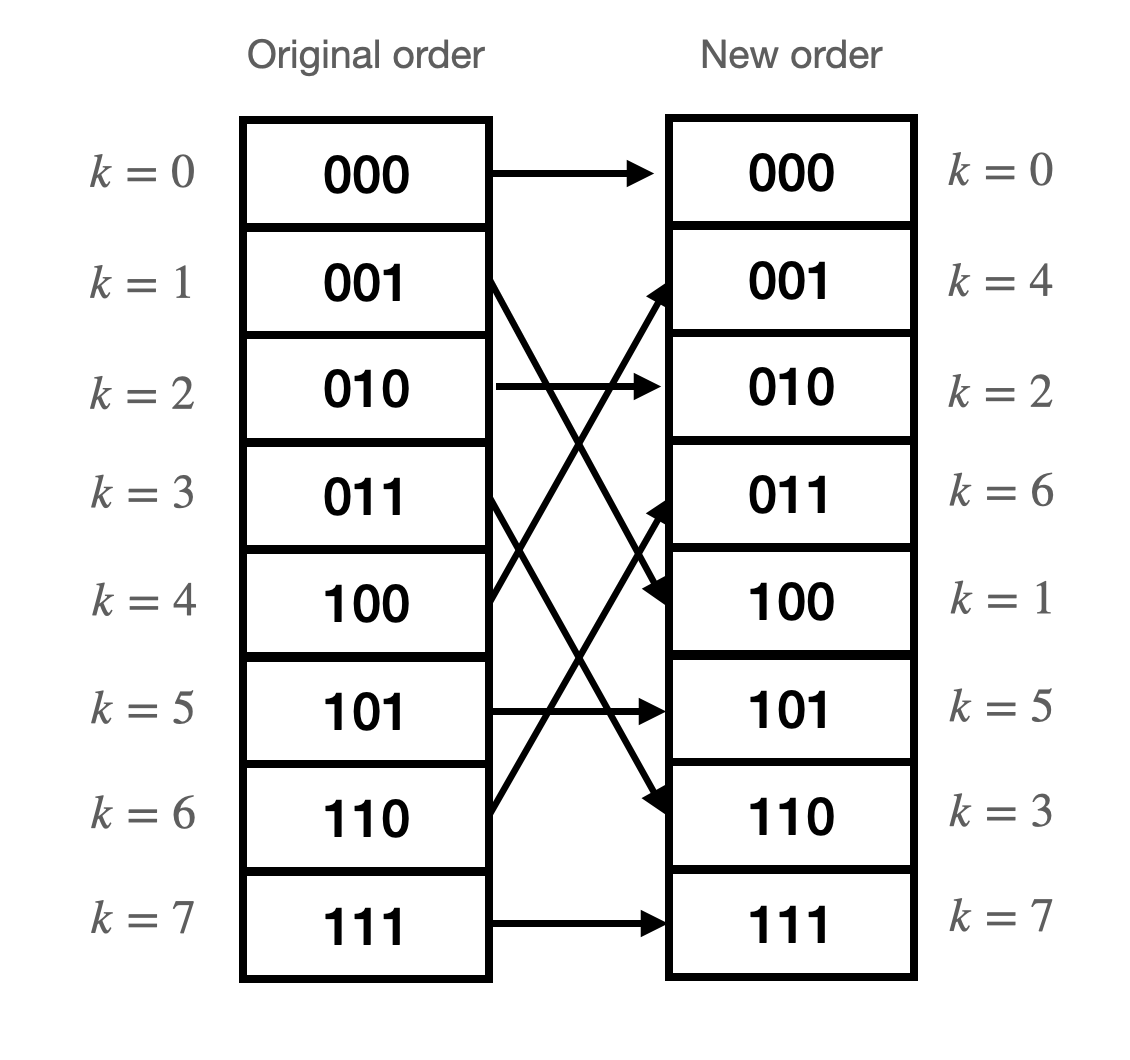
This is a bit reversal permutation.
Multi-point transforms
A single-point transform is simply a reordering of the samples. But how do we construct 2-point transforms from those single-point transforms? And then how do we construct 4-point from those 2-point transforms? And so on? Consider the expression at the core of this recursion:
\begin{align} \underline{c}_m &= \frac{1}{2N}\left[ F^e + e^{-\frac{2\pi i}{2N}m}F^o \right] \end{align}Using the Euler identity $\left(e^{i\theta} = cos{\theta} + i\sin{\theta}\right)$, let us rewrite the above expression using sines and cosines:
\begin{align} \underline{c}_m &= \frac{1}{2N}\left[F_{r}^e + i F_i^e + \left( \cos{\frac{2\pi}{2N}m} - i\sin{\frac{2\pi}{2N}m} \right) \left(F_r^o + i F_i^o\right) \right]\\ &= \frac{1}{2N}\left[F_r^e + i F_i^e + F_r^o \cos{\frac{2\pi}{2N}m} - i F_r^o\sin{\frac{2\pi}{2N}m} + i F_i^o \cos{\frac{2\pi}{2N}m} + F_i^o \sin{\frac{2\pi}{2N}m} \right] \end{align}Separate into real and imaginary components:
\begin{align} \underline{c}_m = \begin{cases} \frac{1}{2N}\left[ F_r^e + F_r^o \cos{\frac{2\pi}{2N}m} + F_i^o \sin{\frac{2\pi}{2N}m}\right] & real\\ \frac{1}{2N}\left[ F_i^e - F_r^o\sin{\frac{2\pi}{2N}m} + F_i^o \cos{\frac{2\pi}{2N}m} \right] & imaginary \end{cases} \end{align}Just to tidy things a bit, let's let $2N \rightarrow N$. Instead of letting $2N$ be the number of samples that we gather, let's let that quantity be represented by the symbol $N$.
\begin{align} \underline{c}_m = \begin{cases} \frac{1}{N}\left[ F_r^e + F_r^o \cos{\frac{2\pi}{N}m} + F_i^o \sin{\frac{2\pi}{N}m}\right] & real\\ \frac{1}{N}\left[ F_i^e + F_i^o \cos{\frac{2\pi}{N}m} - F_r^o\sin{\frac{2\pi}{N}m} \right] & imaginary \end{cases} \end{align}Think about the above expression algorithmically. If we have the odd/even DFT's of length $N$, we can generate the DFT of length $2N$ as follows:
\begin{align} \left(F\right)_{2N} = \begin{bmatrix} \left(F_r\right)_{2N}\\ \left(F_i\right)_{2N}\end{bmatrix} = \begin{bmatrix} \frac{1}{2}\left[ \left(F_r^e\right)_{N} + \left(F_r^o\right)_{N} \cos{\frac{2\pi}{2N}m} + \left(F_i^o\right)_{N} \sin{\frac{2\pi}{2N}m}\right] & (real)\\ \frac{1}{2}\left[ \left(F_i^e\right)_{N} + \left(F_i^o\right)_{N} \cos{\frac{2\pi}{2N}m} - \left(F_r^o\right)_{N}\sin{\frac{2\pi}{2N}m} \right] & (imaginary) \end{bmatrix} & for & m\in [0,2N] \end{align}The notation is getting a bit cumbersome, but the above only says that each DFT of length $N$ can be generated by combining the even/odd DFT's of length $\frac{N}{2}$. Above, we've separated these DFT's into their real/imaginary parts.
This is very close to being an implementable algorithm. There's one more optimization that we can perform. Each time we build a DFT of length $N$ from two DFT's of length $\frac{N}{2}$, the values for $m$ should range from $[0, \frac{N}{2}]$ (the length of each DFT). But! Recall that $\cos{\theta + \pi} = -\cos{\theta}$, and $\sin{\theta + \pi} = -sin{\theta}$. For that reason, we only need to vary $m$ in the range $[0, \frac{N}{4}]$, and we can solve for the values for $m$ in the range $[\frac{N}{4}, \frac{N}{2}]$ by simply flipping the sign of the sine/cosine terms. That is to say:
\begin{align} \underline{c}_{m \in [0, \frac{N}{2}]} &= \begin{cases} \frac{1}{N}\left[ F_r^e + \left(F_r^o \cos{\frac{2\pi}{N}m} + F_i^o \sin{\frac{2\pi}{N}m}\right)\right] & real\\ \frac{1}{N}\left[ F_i^e + \left(F_i^o \cos{\frac{2\pi}{N}m} - F_r^o\sin{\frac{2\pi}{N}m}\right) \right] & imaginary \end{cases}\\ \underline{c}_{m \in [\frac{N}{2}, N]} &= \begin{cases} \frac{1}{N}\left[ F_r^e - \left(F_r^o \cos{\frac{2\pi}{N}\left(m - \frac{N}{2}\right)} + F_i^o \sin{\frac{2\pi}{N}\left(m - \frac{N}{2}\right)}\right)\right] & real\\ \frac{1}{N}\left[ F_i^e - \left(F_i^o \cos{\frac{2\pi}{N}\left(m - \frac{N}{2}\right)} - F_r^o\sin{\frac{2\pi}{N}\left(m - \frac{N}{2}\right)}\right) \right] & imaginary \end{cases} \end{align}This halves the number of trig operations (or table lookups) that we need to implement.
Computational expense for the Cooley-Tukey FFT
Recall that a naive implementation of the discrete Fourier transform was $\mathcal{O}(N^2)$. How much less expensive is the Cooley-Tukey FFT?
In the first step of the Cooley-Tukey FFT (after reordering), we combine $\frac{N}{2}$ pairs of single-point DFT's to obtain $\frac{N}{2}$ two-point DFT's. Then, we combine $\frac{N}{4}$ pairs of two-point DFT's to obtain $\frac{N}{4}$ four-point DFT's. And so on. Each of these combinations takes of order $N$ operations, and we perform $log_2(N)$ of these recombinations. Thus, the complexity of the Cooley-Tukey FFT is $\mathcal{O}(Nlog_2(N))$, assuming that the repordering process is no greater than $Nlog_2(N)$. That's a practical amount of complexity!
8-sample FFT, step-by-step
Sometimes walking through the first few steps of an iteration can add clarity. Let's consider each step of an 8-sample FFT.
Gather data
We begin by gathering 8 samples, each of which has a real and imaginary part. We'll separate these real and imaginary parts into two arrays of length 8. For some applications (e.g. audio sampling), the imaginary array will be all zeroes.
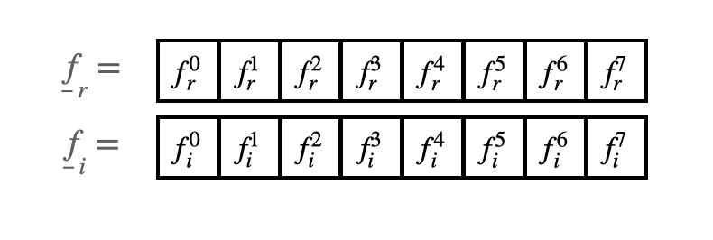
In code, this will look like the following. The real and imaginary components of the samples are stored in separate arrays, each of length NUM_SAMPLES.
#define NUM_SAMPLES         8  // the number of gathered samples (power of two)

fix fr[NUM_SAMPLES] ; // array of real part of samples
fix fi[NUM_SAMPLES] ; // array of imaginary part of samples
For the most efficient code, use fixed point arithmetic.
Single-point transforms (reordering)
We first take the $N=1$ transforms of each of these samples. As discussed previously, this is simply a reordering of the samples.
In code, this looks like the following. Note that there are many algorithms for bit reversal permutations, this is a simple example of one based on bit manipulations.
#define NUM_SAMPLES         8  // the number of gathered samples (power of two)
#define NUM_SAMPLES_M_1  7  // the number of gathered samples minus 1
#define LOG2_NUM_SAMPLES    3  // log2 of the number of gathered samples
#define SHIFT_AMOUNT       13 // length of short (16 bits) minus log2 of number of samples

fix fr[NUM_SAMPLES] ; // array of real part of samples
fix fi[NUM_SAMPLES] ; // array of imaginary part of samples

void bitReversalPermutation() {
    unsigned short m;   // one of the indices being swapped
    unsigned short mr ; // the other index being swapped (r for reversed)
    int t ; // for temporary storage while swapping
    // Code below based on that found here:
    // https://graphics.stanford.edu/~seander/bithacks.html#BitReverseObvious
    for (m=1; m<NUM_SAMPLES_M_1; m++) {
        // swap odd and even bits
        mr = ((m >> 1) & 0x5555) | ((m & 0x5555) << 1);
        // swap consecutive pairs
        mr = ((mr >> 2) & 0x3333) | ((mr & 0x3333) << 2);
        // swap nibbles ...
        mr = ((mr >> 4) & 0x0F0F) | ((mr & 0x0F0F) << 4);
        // swap bytes
        mr = ((mr >> 8) & 0x00FF) | ((mr & 0x00FF) << 8);
        // shift down mr
        mr >>= SHIFT_AMOUNT ;
        // don't swap that which has already been swapped
        if (mr<=m) continue ;
        // swap the bit-reveresed indices
        t = fr[m] ;
        fr[m] = fr[mr] ;
        fr[mr] = t ;
        t = fi[m] ;
        fi[m] = fi[mr] ;
        fi[mr] = t ;
    }
}
After calling the above function, the global arrays fr and fi are reordered.
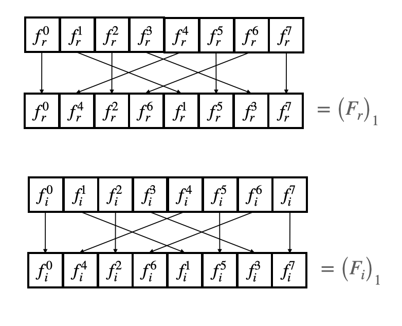
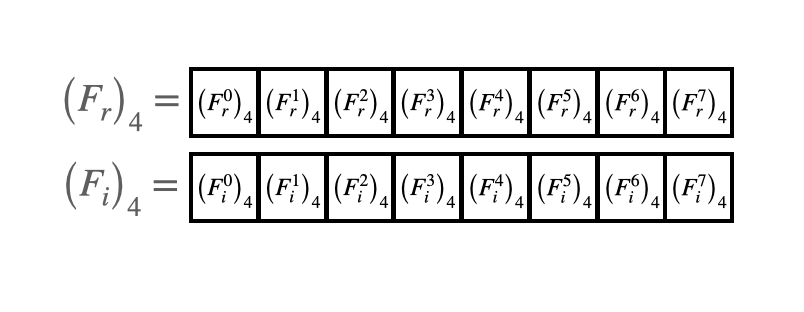
Two-point transforms
From each pair of adjacent points, we calculate the two-point DFT's.
\begin{align} \begin{bmatrix} \left(F_r^0\right)_2 & \left(F_r^1\right)_2\\ \left(F_r^2\right)_2 & \left(F_r^3\right)_2\\ \left(F_r^4\right)_2 & \left(F_r^5\right)_2\\ \left(F_r^6\right)_2 & \left(F_r^7\right)_2 \end{bmatrix} &= \frac{1}{2} \begin{bmatrix} f_r^0 & f_i^0 & f_r^4 & f_i^4 \\ f_r^2 & f_i^2 & f_r^6 & f_i^6 \\ f_r^1 & f_i^1 & f_r^5 & f_i^5 \\ f_r^3 & f_i^3 & f_r^7 & f_i^7 \end{bmatrix} \begin{bmatrix} 1 & 1\\ 0 & 0\\ \cos{\frac{2\pi}{2}(0)} & \cos{\frac{2\pi}{2}(1)}\\ \sin{\frac{2\pi}{2}(0)} & \sin{\frac{2\pi}{2}(1)} \end{bmatrix}\\ \begin{bmatrix} \left(F_i^0\right)_2 & \left(F_i^1\right)_2\\ \left(F_i^2\right)_2 & \left(F_i^3\right)_2\\ \left(F_i^4\right)_2 & \left(F_i^5\right)_2\\ \left(F_i^6\right)_2 & \left(F_i^7\right)_2 \end{bmatrix} &= \frac{1}{2} \begin{bmatrix} f_r^0 & f_i^0 & f_r^4 & f_i^4 \\ f_r^2 & f_i^2 & f_r^6 & f_i^6 \\ f_r^1 & f_i^1 & f_r^5 & f_i^5 \\ f_r^3 & f_i^3 & f_r^7 & f_i^7 \end{bmatrix} \begin{bmatrix} 0 & 0\\ 1 & 1\\ -\sin{\frac{2\pi}{2}(0)} & -\sin{\frac{2\pi}{2}(1)}\\ \cos{\frac{2\pi}{2}(0)} & \cos{\frac{2\pi}{2}(1)} \end{bmatrix} \end{align}Before moving on, we can notice two opportunities for optimization. The first is to realize that, due to the periodicity of the sine and cosine functions mentioned earlier, we need only actually compute the trig functions in the first half of the columns of the rightmost matrix above. The trig functions in column $j + \frac{N}{2}$ where $j<\frac{N}{2}$ are simply the negative of the trig functions in column $j$. So, we could rewrite the above as follows:
\begin{align} \begin{bmatrix} \left(F_r^0\right)_2 & \left(F_r^1\right)_2\\ \left(F_r^2\right)_2 & \left(F_r^3\right)_2\\ \left(F_r^4\right)_2 & \left(F_r^5\right)_2\\ \left(F_r^6\right)_2 & \left(F_r^7\right)_2 \end{bmatrix} &= \frac{1}{2} \begin{bmatrix} f_r^0 & f_i^0 & f_r^4 & f_i^4 \\ f_r^2 & f_i^2 & f_r^6 & f_i^6 \\ f_r^1 & f_i^1 & f_r^5 & f_i^5 \\ f_r^3 & f_i^3 & f_r^7 & f_i^7 \end{bmatrix} \begin{bmatrix} 1 & 1\\ 0 & 0\\ \cos{\frac{2\pi}{2}(0)} & -\cos{\frac{2\pi}{2}(0)}\\ \sin{\frac{2\pi}{2}(0)} & -\sin{\frac{2\pi}{2}(0)} \end{bmatrix}\\ \begin{bmatrix} \left(F_i^0\right)_2 & \left(F_i^1\right)_2\\ \left(F_i^2\right)_2 & \left(F_i^3\right)_2\\ \left(F_i^4\right)_2 & \left(F_i^5\right)_2\\ \left(F_i^6\right)_2 & \left(F_i^7\right)_2 \end{bmatrix} &= \frac{1}{2} \begin{bmatrix} f_r^0 & f_i^0 & f_r^4 & f_i^4 \\ f_r^2 & f_i^2 & f_r^6 & f_i^6 \\ f_r^1 & f_i^1 & f_r^5 & f_i^5 \\ f_r^3 & f_i^3 & f_r^7 & f_i^7 \end{bmatrix} \begin{bmatrix} 0 & 0\\ 1 & 1\\ -\sin{\frac{2\pi}{2}(0)} & \sin{\frac{2\pi}{2}(0)}\\ \cos{\frac{2\pi}{2}(0)} & -\cos{\frac{2\pi}{2}(0)} \end{bmatrix} \end{align}As a second optimization, we can replace the trig calculations with a table lookup. Suppose that we generated an array of length NUM_SAMPLES which contained evenly-spaced sine wave values over a single period. Something like the following:
fix Sinewave[NUM_SAMPLES] ;
for (int i=0; i<NUM_SAMPLES; i++) {
       Sinewave[i] = float2fix(sin(6.283 * ((float)( i) / NUM_SAMPLES) ;
}
Each of the above trig functions is then replaced with a table lookup:
- $\sin{\left(\frac{2 \pi}{2}0\right)}$ $\longrightarrow$
Sinewave[0] - $\cos{\left(\frac{2 \pi}{2}0\right)}$ $\longrightarrow$
Sinewave[0 + NUM_SAMPLES/4](since the cosine curve is 90 degrees out of phase with the sine curve)
This then becomes encoded as follows:
// Length of each FFT being created
istep = 2 ;
// For each element in the single-point FFT's that are being combined . . .
for (m=0; m<1; ++m) {
    // Lookup the trig values for that element
    j = m << 2 ;                        // always 0 since m only attains 0.
    wr =  Sinewave[j + NUM_SAMPLES/4] ; // cos((2pi/2)*0)
    wi = -Sinewave[j] ;                 // sin((2pi/2)*0)
    wr >>= 1 ;                          // divide by two
    wi >>= 1 ;                          // divide by two
    // i gets the index of one of the FFT elements being combined
    for (i=m; i<NUM_SAMPLES; i+=istep) {
        // j gets the index of the FFT element being combined with i
        j = i + 1 ;
        // compute the trig terms (bottom half of the above matrix)
        tr = multfix(wr, fr[j]) - multfix(wi, fi[j]) ;
        ti = multfix(wr, fi[j]) + multfix(wi, fr[j]) ;
        // divide ith index elements by two (top half of above matrix)
        qr = fr[i]>>1 ;
        qi = fi[i]>>1 ;
        // compute the new values at each index
        fr[j] = qr - tr ;
        fi[j] = qi - ti ;
        fr[i] = qr + tr ;
        fr[i] = qi + ti ;
    }

}
These two-point DFT's replace the single-point DFT's in-place in the array, as shown below.
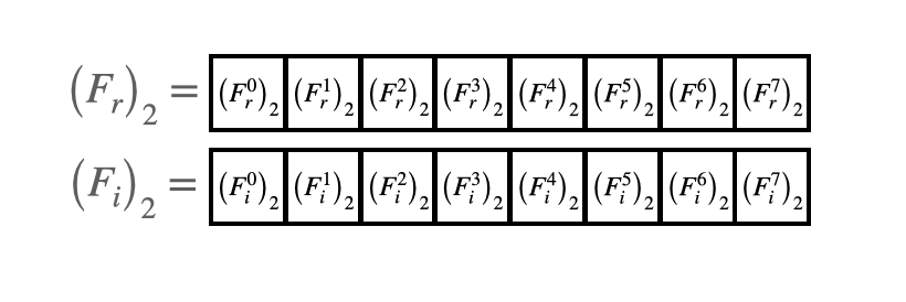
Four-point transforms
We then form four-point DFT's from adjacent pairs of pairs of two-point DFT's. Note that, in the below matrices, I've implemented the periodicity optimization discussed earlier. Namely, that we need only compute the first half of the columns in the matrix of trig functions, and the second half can be calculated by negating the first half.
Each of the above trig functions is then replaced with a table lookup:
- $\sin{\left(\frac{2 \pi}{4}0\right)}$ $\longrightarrow$
Sinewave[0] - $\cos{\left(\frac{2 \pi}{4}0\right)}$ $\longrightarrow$
Sinewave[0 + NUM_SAMPLES/4] - $\sin{\left(\frac{2 \pi}{4}1\right)}$ $\longrightarrow$
Sinewave[2] - $\cos{\left(\frac{2 \pi}{4}1\right)}$ $\longrightarrow$
Sinewave[2 + NUM_SAMPLES/4]
This then becomes encoded as follows:
// Length of each FFT being created
istep = 4 ;
// For each element in the single-point FFT's that are being combined . . .
for (m=0; m<2; ++m) {
    // Lookup the trig values for that element
    j = m << 1 ; // zero the first time through the loop, 2 the second time
    wr =  Sinewave[j + NUM_SAMPLES/4] ; // cos((2pi/4)*[0, 1)
    wi = -Sinewave[j] ;                 // sin((2pi/4)*[0, 1)
    wr >>= 1 ;                          // divide by two
    wi >>= 1 ;                          // divide by two
    // i gets the index of one of the FFT elements being combined
    for (i=m; i<NUM_SAMPLES; i+=istep) {
        // j gets the index of the FFT element being combined with i
        j = i + 2 ;
        // compute the trig terms (bottom half of the above matrix)
        tr = multfix(wr, fr[j]) - multfix(wi, fi[j]) ;
        ti = multfix(wr, fi[j]) + multfix(wi, fr[j]) ;
        // divide ith index elements by two (top half of above matrix)
        qr = fr[i]>>1 ;
        qi = fi[i]>>1 ;
        // compute the new values at each index
        fr[j] = qr - tr ;
        fi[j] = qi - ti ;
        fr[i] = qr + tr ;
        fr[i] = qi + ti ;
    }
}
As before, the four-point DFT's then replace the two-point DFT's in the arrays:
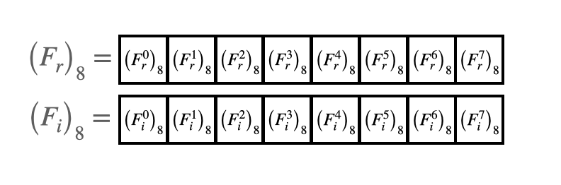
8-point transform
Finally, the two adjacent 4-point transforms are combined to an 8-point transform. (Note the transpose on the first vector. Transposed just so it fits on the page a bit more nicely). Note that, in the below matrices, I've implemented the periodicity optimization discussed earlier. Namely, that we need only compute the first half of the columns in the matrix of trig functions, and the second half can be calculated by negating the first half.
Each of the above trig functions is then replaced with a table lookup:
- $\sin{\left(\frac{2 \pi}{8}0\right)}$ $\longrightarrow$
Sinewave[0] - $\cos{\left(\frac{2 \pi}{8}0\right)}$ $\longrightarrow$
Sinewave[0 + NUM_SAMPLES/4] - $\sin{\left(\frac{2 \pi}{8}1\right)}$ $\longrightarrow$
Sinewave[1] - $\cos{\left(\frac{2 \pi}{8}1\right)}$ $\longrightarrow$
Sinewave[1 + NUM_SAMPLES/4] - $\sin{\left(\frac{2 \pi}{8}2\right)}$ $\longrightarrow$
Sinewave[2] - $\cos{\left(\frac{2 \pi}{8}2\right)}$ $\longrightarrow$
Sinewave[2 + NUM_SAMPLES/4] - $\sin{\left(\frac{2 \pi}{8}3\right)}$ $\longrightarrow$
Sinewave[3] - $\cos{\left(\frac{2 \pi}{8}3\right)}$ $\longrightarrow$
Sinewave[3 + NUM_SAMPLES/4]
This then becomes encoded as follows:
// Length of each FFT being created
istep = 8 ;
// For each element in the single-point FFT's that are being combined . . .
for (m=0; m<4; ++m) {
    // Lookup the trig values for that element
    j = m << 0 ; // assumes values 0, 1, 2, 3
    wr =  Sinewave[j + NUM_SAMPLES/4] ; // cos((2pi/8)*[0, 1, 2, 3])
    wi = -Sinewave[j] ;                 // sin((2pi/8)*[0, 1, 2, 3])
    wr >>= 1 ;                          // divide by two
    wi >>= 1 ;                          // divide by two
    // i gets the index of one of the FFT elements being combined
    for (i=m; i<NUM_SAMPLES; i+=istep) {
        // j gets the index of the FFT element being combined with i
        j = i + 4 ;
        // compute the trig terms (bottom half of the above matrix)
        tr = multfix(wr, fr[j]) - multfix(wi, fi[j]) ;
        ti = multfix(wr, fi[j]) + multfix(wi, fr[j]) ;
        // divide ith index elements by two (top half of above matrix)
        qr = fr[i]>>1 ;
        qi = fi[i]>>1 ;
        // compute the new values at each index
        fr[j] = qr - tr ;
        fi[j] = qi - ti ;
        fr[i] = qr + tr ;
        fr[i] = qi + ti ;
    }
}
Which, as before, replaces the 4-point FFT's:
From the above step-by-step example, we can generalize to create code that will calculate FFT's for any power-of-two number of samples.
Generalized code
We can generalize the above code for a number of samples which is any power of two:
#define NUM_SAMPLES           // the number of gathered samples (power of two)
#define NUM_SAMPLES_M_1    // the number of gathered samples minus 1
#define LOG2_NUM_SAMPLES      // log2 of the number of gathered samples
#define SHIFT_AMOUNT         // length of short (16 bits) minus log2 of number of samples

fix fr[NUM_SAMPLES] ; // array of real part of samples (WINDOWED)
fix fi[NUM_SAMPLES] ; // array of imaginary part of samples (WINDOWED)

void FFTfix(fix fr[], fix fi[]) {

    unsigned short m;   // one of the indices being swapped
    unsigned short mr ; // the other index being swapped (r for reversed)
    fix tr, ti ; // for temporary storage while swapping, and during iteration

    int i, j ; // indices being combined in Danielson-Lanczos part of the algorithm
    int L ;    // length of the FFT's being combined
    int k ;    // used for looking up trig values from sine table

    int istep ; // length of the FFT which results from combining two FFT's

    fix wr, wi ; // trigonometric values from lookup table
    fix qr, qi ; // temporary variables used during DL part of the algorithm

    //////////////////////////////////////////////////////////////////////////
    ////////////////////////// BIT REVERSAL //////////////////////////////////
    //////////////////////////////////////////////////////////////////////////
    // Bit reversal code below based on that found here:
    // https://graphics.stanford.edu/~seander/bithacks.html#BitReverseObvious
    for (m=1; m<NUM_SAMPLES_M_1; m++) {
        // swap odd and even bits
        mr = ((m >> 1) & 0x5555) | ((m & 0x5555) << 1);
        // swap consecutive pairs
        mr = ((mr >> 2) & 0x3333) | ((mr & 0x3333) << 2);
        // swap nibbles ...
        mr = ((mr >> 4) & 0x0F0F) | ((mr & 0x0F0F) << 4);
        // swap bytes
        mr = ((mr >> 8) & 0x00FF) | ((mr & 0x00FF) << 8);
        // shift down mr
        mr >>= SHIFT_AMOUNT ;
        // don't swap that which has already been swapped
        if (mr<=m) continue ;
        // swap the bit-reveresed indices
        tr = fr[m] ;
        fr[m] = fr[mr] ;
        fr[mr] = tr ;
        ti = fi[m] ;
        fi[m] = fi[mr] ;
        fi[mr] = ti ;
    }

    //////////////////////////////////////////////////////////////////////////
    ////////////////////////// Danielson-Lanczos //////////////////////////////
    //////////////////////////////////////////////////////////////////////////
    // Adapted from code by:
    // Tom Roberts 11/8/89 and Malcolm Slaney 12/15/94 malcolm@interval.com
    // Length of the FFT's being combined (starts at 1)
    L = 1 ;
    // Log2 of number of samples, minus 1
    k = LOG2_NUM_SAMPLES - 1 ;
    // While the length of the FFT's being combined is less than the number of gathered samples
    while (L < NUM_SAMPLES) {
        // Determine the length of the FFT which will result from combining two FFT's
        istep = L<<1 ;
        // For each element in the FFT's that are being combined . . .
        for (m=0; m<L; ++m) {
            // Lookup the trig values for that element
            j = m << k ;                         // index of the sine table
            wr =  Sinewave[j + NUM_SAMPLES/4] ; // cos(2pi m/N)
            wi = -Sinewave[j] ;                 // sin(2pi m/N)
            wr >>= 1 ;                          // divide by two
            wi >>= 1 ;                          // divide by two
            // i gets the index of one of the FFT elements being combined
            for (i=m; i<NUM_SAMPLES; i+=istep) {
                // j gets the index of the FFT element being combined with i
                j = i + L ;
                // compute the trig terms (bottom half of the above matrix)
                tr = multfix(wr, fr[j]) - multfix(wi, fi[j]) ;
                ti = multfix(wr, fi[j]) + multfix(wi, fr[j]) ;
                // divide ith index elements by two (top half of above matrix)
                qr = fr[i]>>1 ;
                qi = fi[i]>>1 ;
                // compute the new values at each index
                fr[j] = qr - tr ;
                fi[j] = qi - ti ;
                fr[i] = qr + tr ;
                fi[i] = qi + ti ;
            }
        }
        --k ;
        L = istep ;
    }
}
An example implementation
This code implements the above FFT algorithm on a Raspberry Pi Pico (RP2040). For more details, see this webpage.
What about the inverse FFT?
Recall our expressions for the forward and reverse discrete Fourier transfoms from previously:
\begin{align} f_k = \sum_{n=0}^{2N-1} \underline{c}_n e^{\frac{2\pi n i}{T_0}t_k} \end{align}where
\begin{align} \underline{c}_m = \frac{1}{2N}\sum_{k=0}^{2N-1} e^{-\frac{2\pi m i}{T_0}t_k} f_k \end{align}From these two expressions, we can see that the inverse FFT is identical to the forward FFT except for the leading scaling term and the sign of the exponential. So, the algorithm for the ifft is identical to that for the forward fft except that there is no sign reversal on the assignment for wi, and qr and qi are not right-shifted by 1.
Future topics
- Parallelization
- 2D FFT's