About this document
This document was assembled for students in ECE 4760, who are asked to construct and control a constrained drone like the one described below. I used the RP2040 for the demo videos rather than a PIC32 so that I could make use of the VGA screen for visualizations.
This document focuses on building a phenomenological understanding of PID controllers through demos. A second document will focus on building an analytical understanding of these controllers. The hope is that this document will help you debug your system based on the behavior that you observe in lab, and the other document will help you understand that behavior.
Video discussion of the content on this page
System under consideration
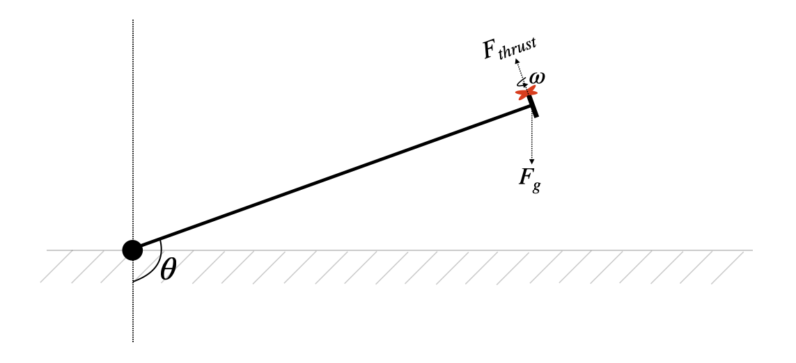
Consider the system illustrated below. There is a drone motor rigidly attached to the end of a lever arm. The other end of this lever arm is attached to a low-torque potentiometer. As the motor spins increasingly quickly ($\omega$ rad/sec), the thrust that it generates ($F_{thrust}$) exceeds the force of gravity ($F_g$) and lifts the arm to increasingly large angles $\theta$ away from the vertical. This is the system that we will build and control in ECE 4760. The user will specify a target angle, $\theta$, and a PID controller will control the motor speed to drive the arm to that angle. This document aims to systematically build an intuition for the system and for the controller that we'll use to control this system.
Open loop control
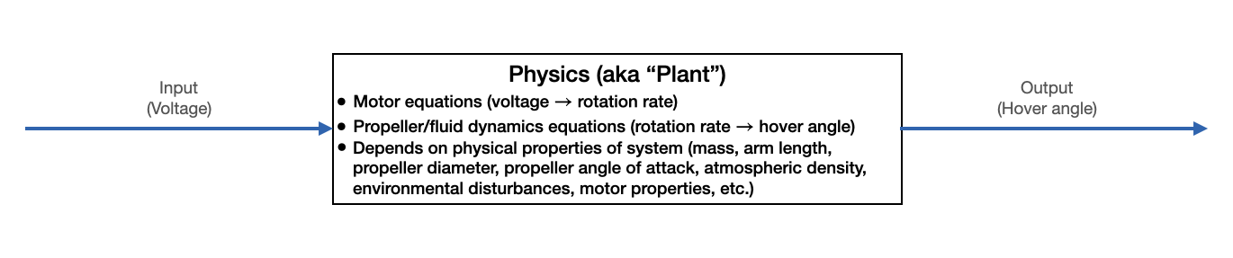
One strategy for controlling this system is open loop control. The control input to the motor is a voltage. 0 voltage means that the motor is not spinning, and increasing voltages lead to increasing motor speeds (up to some saturation speed). So, for each possible input voltage, we could solve for the output motor speed associated with that voltage. With a little physics, you could then solve for the angle $\theta$ that will be achieved for each input voltage. In principle, this reduces the control problem to a lookup table. For a particular target angle, the program would lookup the control voltage associated with that angle and blindly apply that voltage to the motor. This is illustrated in the block diagram below. The open-loop system takes a control input, physics happens, and there is an output. The control input is not adjusted based on the output. What's the problem with this?
The problem is that this makes the accuracy of our system extremely sensitive to the conditions under which it was modeled and/or calibrated. If we were to run our system in Colorado, we'd find that we'd consistently come up short of our target angles (since the atmospheric density would be less). If we bumped our setup and the motor tilted slightly, we'd start seeing errors. As the motor warms or ages and its properties change, we'd see errors. Any load on the system, any change in the system, or any change in the environment would induce an error. For every desired hover angle, there does exist a motor speed that will achieve that angle. But how well can you know that motor speed, and how constant is it over time and from environment to environment?
Please note! Open-loop control is a completely reasonable approach for many situations, particularly those where the system is well understood and in a highly stable environment. It is just not a good approach for our particular system.
Closing the loop
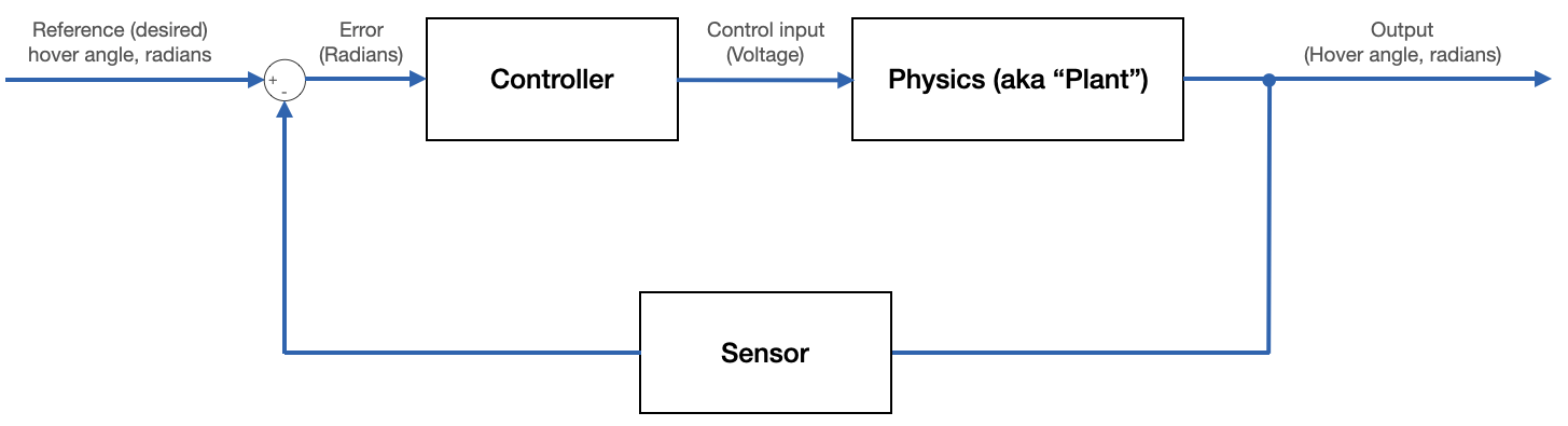
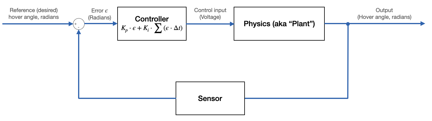
We want for our system to make adjustments on its own in order to move to the desired hover angle. In order to achieve this, we close the loop. We sense the current output of the system (in our case, hover angle) and compare it with the desired hover angle. This error between the current and desired hover angles is then used to adjust the control input to the system. In this way, the system can move itself toward the desired state.
The controller takes the error signal (which is in the same units as the output of the plant, on our case radians) and converts it to the units that are required for the control input (in our case, voltage). Furthermore, the controller must convert this error signal in such a way that the input into the motor drives it to the desired hover angle. There are many varieties of controllers. We will consider a particular variety called PID controllers.
We are considering PID controllers because they are everywhere. These are, by far, the most ubiquitous controllers used in industry.
PID Controllers
"PID" is an acronym that stands for Proportional Integral Derivative. As the name suggests, this controller is composed of three terms that are summed together to form the control input. The first of those terms is proportional to the current error between the measured and desired output, the next is proportional to the integral of that error, and the third is proportional to the rate of change of that error. We'll consider each separately and build up some intuition about how each affects the system.
Proportional term
To start building up a controller, we might first consider doing something quite simple. Suppose that our controller took the error signal as an input, scaled it by some constant $K_p$, and used that scaled value as the input voltage to our motor.
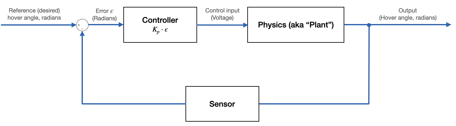
Intuitively, this feels like a step in the right direction. If our desired angle is much greater than our current measured angle then the error will be large, so the control input will be large and the motor will spin fast to move toward the desired hover angle. This is illustrated in the plot below. But! There's a problem.

The motor is fighting against gravity in order to lift the arm to a desired angle. If the error between the desired and measured angles is great enough, then the motor will spin quickly enough to lift the arm toward the desired angle. However, this error will decrease as the motor approaches the desired angle. As the error decreases, the input voltage to the motor will also decrease. As some point, the thrust from the motor will be in equilibrium with the force of gravity and the arm will stop moving with some steady-state error (see the video below). We could decrase this error by increasing our gain $K_p$, but it will never go away completely. And increasing $K_p$ too much can introduce another problem.
If we make $K_p$ too large, then the motor will be moving very quickly until it is very near to the desired hover angle. As a consequence, the arm will have acquired significant velocity and will overshoot the desired hover angle. The same thing will then happen in the opposite direction, and the motor will oscillate around the desired angle (see video below). Not good! We can fix this problem by augmenting our controller with another term.
Integral term
A proportional controller only looks at the current output error. It does not know anything about the history of that error. In order to eliminate the steady-state errors that are produced by a strictly proportional controller, we need a mechanism by which the controller can notice that it has a steady-state error and increase the motor speed to correct this error. We do that by including an integral term in our controller.
The integral term does not scale the instantaneous error between the current and desired outputs. Instead, it scales the integral of that error over time. It is maintaining an accumulating sum of the time history of errors (positive error increases the sum, negative error decreases the sum). This accumulated error is then scaled and added to the proportional term, as shown in the block diagram below.
By the way: note that careful selection of units for time makes $\Delta t = 1$.
This term will eliminate steady state error. Consider the case that our arm has come to rest with some small steady-state error below the desired hover angle. The contribution from the proportional term in the controller will be small because the instantaneous error is small, but that small instantaneous error will accumulate over time. As this error accumulates, the contribution from the integral term in the controller increases and the motor speed will increase until it achieves the desired hover angle.
There are some things to be cautious about associated with this integral term that will be covered in a later section.
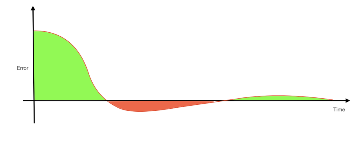
This takes care of the steady-state error, but we still may have a problem with overshoot! Depending on the path that we took to the desired hover angle, it may be the case that the integrator term has accumulated enough error to go passed the desired angle. In order for this term's contribution to decrease, but must overshoot so that the error is negative and the contribution from this term decreases. So, we've eliminated steady-state error, but we may still have overshoot and ringing, particularly if we're trying to make our system respond quickly.
Derivative term
The proportional term looks at the current error, the integral term looks at the past error, and the derivative term makes guesses about how the error will change in the future. This term scales the rate of change of the error, as shown in the block diagram below.
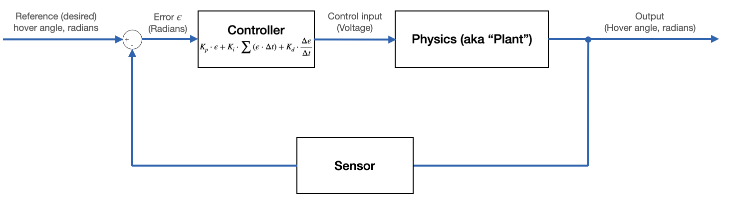
By the way: note that careful selection of units for time makes $\Delta t = 1$.
If the error is decreasing very quickly (the motor is speeding toward the desired hover angle), the derivative of the error will be large and negative, as shown below. As such, the contribution from the derivative term of the PID controller will work against the proportional and integral terms, slowing the speed of the motor. This effect can be balanced against the proportional effect to control the system such that it is fast, but with overshoot that is within the requirements for your application. In some applications (like ours) some overshoot is fine. In other applications (landing a rocket on a barge, perhaps), overshoot is very destructive indeed.

There are two videos below. One shows an untuned PID controller with significant overshoot/ringing. The other shows a highly tuned controller.
Common problems with PID controllers (and their solutions)
Integrator windup
Consider the integrator term of the PID controller. Recall that this term's contribution to the control input is proportional to the error accumulated over time. The behavior that we desire is for this term to increase in value for as long as the error is positive, to remain constant when the error is zero (i.e. we are hovering at the desired hover angle), and to decrease when the error is negative (i.e. we've overshot the desired hover angle). Over time, we expect that this will stabilize to a constant value that keeps the arm at precisely the commanded angle. But, this term can create problems in some situations.
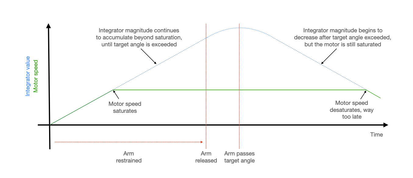
Consider the situation where the arm is hanging straight down, you command it to hover horizontally, but you physically restrain it for a few seconds so that it doesn't move. What will happen?
The proportional term of the PID controller will stay constant for as long as the arm is held in place. What will happen to the integral term? It will continue to accumulate for as long as you restrain the arm. The contribution from the integral term will grow until the motor is saturated, and then it will continue to grow beyond even the value which saturates the motor. It will only begin to decrease once the arm is released and moves past the commanded hover angle. But if you've restrained the arm for too long, the motor will stay saturated for a long time after the arm moves past the desired angle. The integrator term will have accumulated so much magnitude that it will take a long time for it to come back down and for the motor to slow. In the meantime, your system will have blown by your commanded angle and perhaps damaged itself. See the demo video below.
This problem is called integrator windup. There are a few solutions to this problem, but the simplest is to clamp this term at some maximum value.
These are the conditions under which we prevent the integrator from accumulating any more value:
- The controller output is saturated.
- The sign of the controller output is the same as the sign of the error (i.e. the integrator is making the situation worse).
As soon as the error switches sign, we unclamp the integrator term so that it immediately starts to decrease, limiting overshoot. It's a good idea to be a bit conservative with your clamping limits, don't make them the same as the saturation values for your actuators. Demo video below of integrator windup prevention with clamping.
Derivative noise amplification
The block diagrams above omit something extremely important: noise. This noise exists at all frequencies and can come from both the environment (think turbulence) and from your sensors.
This has serious implications for our PID controller because we are differentiating the error. High-frequency noise in the error signal will be amplified by the derivative term in the controller and can have adverse effects on the system. Why is high-frequency noise amplified by the derivative term? Noise is just a collection of additively combined sine waves. Consider the equation for a sine wave:
\begin{align} y(t) = A \sin{\left(\omega \cdot t + \phi\right)} \end{align}If we differentiate this, we get:
\begin{align} \frac{dy}{dt} = A\omega \sin{\left(\omega \cdot t + \phi + 90^{\circ}\right)} \end{align}So, if $\omega> 1$ rad/sec, then the amplitude of the derivative is greater than the amplitude of the original signal. The larger the frequency, the larger the amplitude. If we don't do anything about this, then these noise contributions to the derivative term will create noise in our controller. At best, this creates some jitter in the output (as shown in the video below). At worst, it will destabilize the system.
The video below shows the arm jittering due to noisy input to the derivative term of the PID controller.
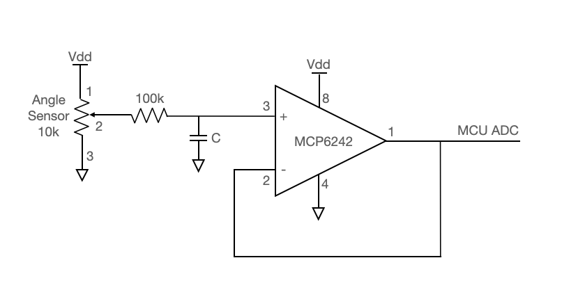
We solve this problem with a lowpass filter that attenuates high frequency input to the controller and passes low-frequency signal. Such a filter could be implemented in hardware or software. An opamp circuit like the one shown below, placed between the sensor and the ADC input of the microcontroller, will attenuate this noise. Choose R and C appropriately for the bandwidth of your system.
Small derivative signal
There's another way that noise can affect the derivative term of the PID controller. Consider the speed of the system vs. the speed of the controller.
I am running this controller at 1 KHz. This means that I am sampling the ADC 1000 times per second, and computing the derivative of the error signal 1000 times per second. From one sample to the next, how much should we expect for the ADC measurement to change, even when the arm is swinging as fast as it can manage?
If we turn the motor on full speed, it will rotate from vertical to horizontal in approximately 0.2 seconds. When hanging vertically, I read an ADC value off the potentiometer of 970 (using the 12-bit DAC on the RP2040). At horizontal, I measure an ADC value of 2040. This implies that the fastest that the ADC measurements are changing is 1070 ADC units in 0.2 seconds, or at a rate of approximately 5-6 ADC units per measurement. The RP2040 has only 9 effective bits, so changes this small are swallowed by noise.
This is mitigated by being a bit careful when numerically esimating the derivative. There are a few options, but a simple one is to look a few samples back when doing the Euler approximation to the derivative. That is, instead of computing the derivative as:
\begin{align} \text{derivative} \approx \text{error}(n) - \text{error}(n-1) \end{align}Instead compute it as:
\begin{align} \text{derivative} \approx \text{error}(n) - \text{error}(n-x) \end{align}where $x$ is large enough for the signal to drive the difference in error measurements rather than noise. $x=4$ worked for me.
Tuning the system
You will end up manually testing and tuning the $K_p$, $K_i$ and $K_d$ gains, but we can come up with some reasonable starting places.
Initial guess for Kp
Suppose that the arm is hanging straight down, and we send it a command to hover horizontally. On the RP2040, straight down corresponds to an ADC reading of 970, and horizontal corresponds to an ADC reading of 2040. This will give us an initial error of 2040-970 = 1070 ADC units.
Probably, we'd like for the motor to turn on full throttle when it sees this error. This can give us a reasonable guess for the proportional gain $K_d$. Suppose that we are running the CPU at 25MHz, so that a 1KHz PWM signal accepts duty cycles in the range of 0-25000 CPU cycles. When the system sees the initial error of 1070 ADC units, we'd like for it to set the PWM duty cycle to about 25000. That implies a $K_p$ of about $\frac{25000}{1070} \approx 23$. More to the point, it suggests a $K_p$ value on the order of 10's rather than 100's or 1000's. Perhaps we start with 10.
Suppose instead that we were running our CPU at 40MHz and we were using a 10-bit DAC so that straight down corresponded to a measurement of about 250 ADC units and horizontal corresponded to about 500. At 40MHz, a 1000 KHz PWM accepts duty cycles in the range 0-40000. If we want the motor on full throttle when it sees an error of 250 ADC units, this suggest a $K_p$ of approximately $\frac{40000}{250} = 160$. In this case, we expect $K_p$ to be on the order of 100's. Perhaps we start with 100.
Initial guess for Kd
In a previous section, we discussed that, when rotating at its fastest, we expect for the ADC measurements to change at about 5-6 units per measurement for the 12-bit DAC on the RP2040. The derivative term of the PID controller scales these differences in measurements by the derivative gain $K_d$. We'd like for the contribution from this term to be non-negligible, which suggests that we'd like for it to be of approximately the same magnitude as the proportional term. These measurement differences are 2-3 orders of magnitude smaller than the error measurements used by the proportional term (depending how many samples back you look for the derivative approximation, see previous section). So, we expect for $K_d$ to be 2-3 orders of magnitude larger than $K_p$. In the range of 1000's-10000's. Perhaps you start with around 1000.
Initial guess for Ki
As with $K_d$, we'd like for the contribution from the integral term to be of approximately the same magnitude as that from the proportional term. We need to be careful with the integral term, however! It can destabilize the system if it is too big.
The integral term is summing errors, and those errors will (initially) be on the order of 1000 ADC units. So, $K_i$ will be small compared to $K_p$ and $K_d$. Perhaps you start with a value of $\frac{1}{32}$ and increase as necessary to eliminate steady-state error. It's a good idea to make $K_i$ a power of 2 so that you can use shift operations and maintain integer arithmetic in all your control calculations.
Tuning
Start with just a proportional gain. Increase this gain until the system is on the edge of stability (oscillating) and then add some derivative gain to suppress overshoot and oscillation. Get the system to respond quickly by increasing $K_p$, and suppress overshoot using $K_d$. Then add a bit of integral gain $K_i$ to eliminate steady state error.