Analytical Introduction to PID controllers
V. Hunter Adams
from IPython.core.display import HTML
HTML('''<script>
code_show=true;
function code_toggle() {
 if (code_show){
 $('div.input').hide();
 } else {
 $('div.input').show();
 }
 code_show = !code_show
}
$( document ).ready(code_toggle);
</script>
<form action="javascript:code_toggle()"><input type="submit" value="Click here to toggle on/off the raw code."></form>''')
About this document
This document was assembled for students in ECE 4760, who are asked to construct and control a contrained drone like the one described below.
A separate document focuses on building a phenomenological understanding of PID controllers through demos. This document focuses on building an analytical understanding of these controllers. The hope is that the phenomenological document will help you debug your system based on the behavior that you observe in lab, and this one will help you understand that behavior.
- Phenomenological PID page (useful for debugging in lab)
System under consideration
Consider the system illustrated below. There is a drone motor rigidly attached to the end of a lever arm. The other end of this lever arm pivots about a hinge. There is an accelerometer/gyro rigidly attached to the arm, with which we estimate the arm angle with a complementary filter.
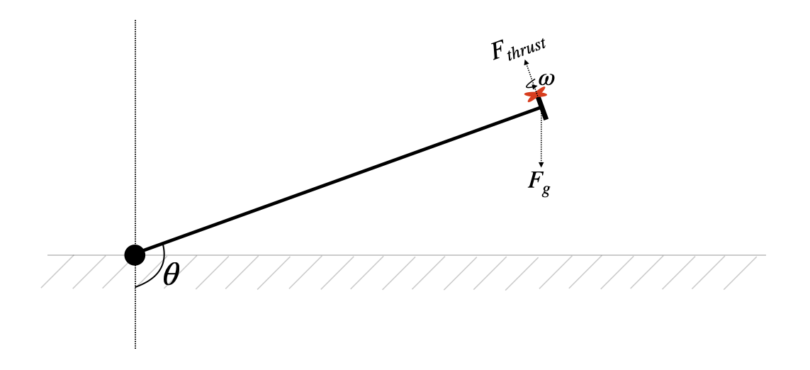
As the motor spins increasingly quickly ($\omega$ rad/sec), the thrust that it generates ($F_{thrust}$) exceeds the force of gravity ($F_g$) and lifts the arm to increasingly large angles $\theta$ away from the vertical. This is the system that we will build and control in ECE 4760. The user will specify a target angle, $\theta$, and a PID controller will control the motor speed to drive the arm to that angle. This document aims to systematically build an intuition for the system and for the controller that we'll use to control this system.
Modeling the motor
Mechanical motor model
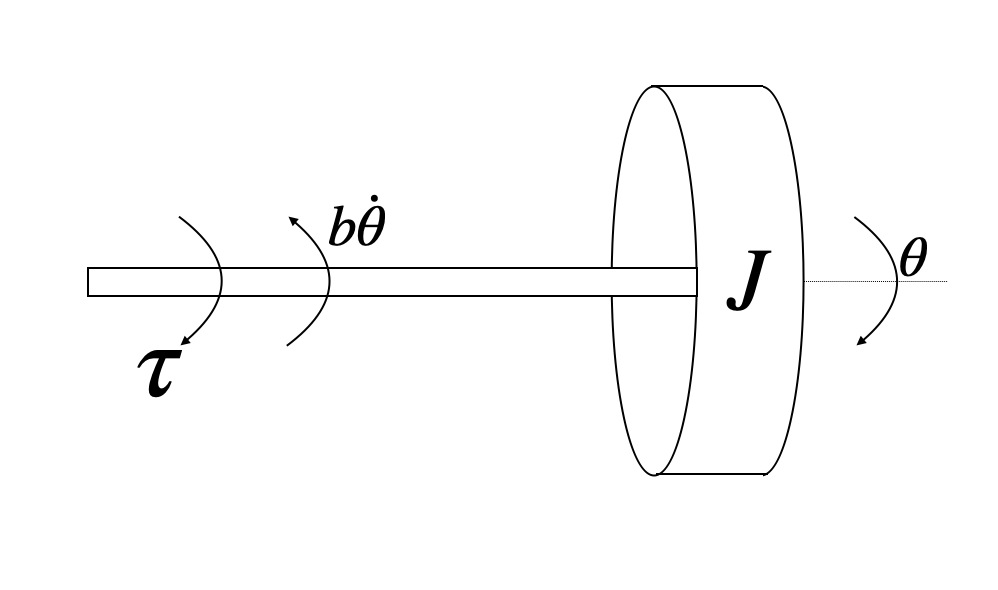
We can mechanically model the motor as an inertial mass spinning about a shaft. This inertial mass has some moment of inertia $J$. An external torque, $\tau$, rotates the shaft by some angle $\theta$. As the shaft rotates, it experiences drag that is proportional to its rotation speed, $b\dot{\theta}$. The net torque on the shaft produces an angular acceleration according to $\sum \tau = J\ddot{\theta}$.
All of these can be combined into the following torque-balance equation:
Electrical motor model
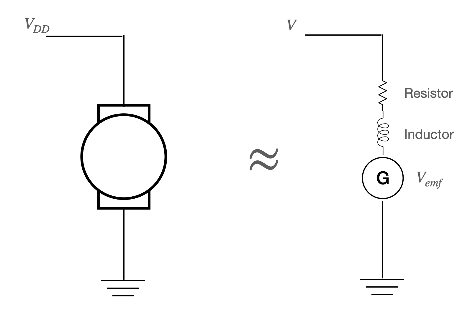
A motor works by placing current through a wire coil armature. This armature rests in a static magnetic field, which exerts a Lorentz force on the current-carrying armature. As the armature spins, current is also induced in the opposite direction. As such, the electrical model for a DC motor is a resistor, inductor, and back-emf voltage sorce in series.
Using Kirchoff's voltage law, we arrive at an expression which relates the voltage among all the components in the electrical model of our motor:
\begin{align} V - Ri - L\frac{di}{dt} - V_{emf} = 0 \end{align}Rewriting $V_{emf}$
Within the operating limits of the motor (i.e. not at saturation), there is an approximately linear relationship between the voltage applied to the motor ($V$) and the rotation rate ($\dot{\theta}$). The slope of this line can be established experimentally for a particular motor, but we will use some general proportionality constant $K_v$.
\begin{align} \dot{\theta} = K_v V \end{align}This is an expression that gives us rotation speed as a function of applied voltage. By rearranging this equation, we can solve for $V_{emf}$, which is generated voltage as a function of motor speed:
\begin{align} V_{emf} = \frac{1}{K_v} \dot{\theta} \end{align}For tidyness, we'll define $\frac{1}{K_v} \equiv K_e$, giving us the expression:
\begin{align} V_{emf} = K_e \dot{\theta} \end{align}Substituting back into the electrical motor model yields:
\begin{align} V - Ri - L\frac{di}{dt} - K_e \dot{\theta} = 0 \end{align}Rewriting $\tau$
We've seen that the output speed of the motor is proportional to applied voltage. Similarly, the output torque of the motor is proportional to current through the motor. The constant of proportionality is the torque constant $K_t$.
\begin{align} \tau = K_t i \end{align}Substituting into the mechanical motor model equation yields:
\begin{align} K_t i - b\dot{\theta} = J\ddot{\theta} \end{align}Simplifying $K_t$ and $K_e$
Note that in SI units, $K_t = K_e$. So, we'll define some term $K \equiv K_t = K_e = \frac{1}{K_v}$. Substituting this into our electrical and mechanical models for the motor yields:
\begin{align} K i - b\dot{\theta} &= J\ddot{\theta}\\ 0&= V - Ri - L\frac{di}{dt} - K \dot{\theta} \end{align}Laplace transforms
Take the Laplace transform of each differential equation.
Transfer function
Let us define $s\Theta(s) \equiv \Omega(s)$ and substitute/rearrange the above two equations to get our transfer function:
Bode plot
Let's take some reasonable guesses at these motor parameters and create a Bode plot for the motor response.
from scipy import signal
import matplotlib.pyplot as plt
import numpy
%matplotlib inline
plt.rcParams['figure.figsize'] = [20, 5]

J = 4.5e-9
b = 1e-8
K = 6.3e-4
R = 2.6
L = 5.0e-3

sys = signal.TransferFunction([K], [J*L, (J*R + b*L), b*R + K**2.])
w, mag, phase = signal.bode(sys)

plt.figure()
plt.title('Bode plot for motor')
plt.semilogx(w, mag)    # Bode magnitude plot
plt.grid('on')
plt.ylabel('dB')
plt.figure()
plt.semilogx(w, phase)  # Bode phase plot
plt.grid('on')
plt.xlabel('Rad/sec')
plt.ylabel('Degrees')
plt.show()


Step response
The motor's step response to a 1V square input:
lti = signal.lti([K], [J*L, (J*R + b*L), b*R + K**2.])
t, y = signal.step2(lti)
plt.title('Step response of motor');plt.plot(t,y)
plt.grid('on')
plt.xlabel('sec'); plt.ylabel('Rad/sec');plt.show()

Making some observations
What you will notice is that the motor looks like a 2-pole lowpass filter with a cutoff frequency that is quite high. When we apply a square wave input to the motor, the output speed of the motor increases effectively instantaneously from the standpoint of the pendulum. We're about to look at the pendulum dynamics, but we'll see that the pendulum is way slower than the motor. This means that the time constants are all dominated by the lowpass characteristics of the pendulum, and by the resonance of the pendulum.
Modeling the pendulum physics
We will solve for the pendulum equation of motion by setting up a torque balance. There are three contributions to the torque on the pendulum: gravity, friction, and thrust. Thrust is always pointing in the direction that the motor is pointing, and gravity is always pointing toward the center of Earth, and friction acts opposite the direction of motion.
Thrust
Thrust is approximately proporitonal to the square of the rotor rotation speed. The constant of proportionality depends on lots of stuff (properties of the propeller, the fluid, etc.), but we'll just call it $K_T$ and play with it in simulation until we get a response that looks pretty good.
\begin{align} \tau_{thrust} &= K_T \omega^2 L \end{align}Gravity
The force from gravity is always toward the center of the Earth, so we must account for the angle of the beam in our torque calculation.
\begin{align} \tau_g &= m g L \sin{\theta} \end{align}
Friction
And the torque from friction is proportional to the rotation rate, $\dot{\theta}$:
\begin{align} \tau_f &= K_f \dot{\theta} \end{align}Equation of motion
We know that the net torque equals the moment of inertia times the angular acceleration, as shown below:
\begin{align} \sum \tau &= J \ddot{\theta} \end{align}If we assume that the mass of the beam is negligible compared to the mass of the motor, then the moment of inertia is simply $J=mL^2$. Thus:
\begin{align} \sum \tau = m L^2 \ddot{\theta} \end{align}Substitute the torque expressions:
\begin{align} \tau_{thrust} - \tau_g - \tau_f &= m\cdot L^2 \cdot \ddot{\theta}\\ K_T \omega^2 L - m g L \sin{\theta} - K_f \dot{\theta} &= m L^2 \ddot{\theta} \end{align}Solve for the angular acceleration:
Linearization
That's a nonlinear equation! For sake of deploying some standard linear analysis, let's linearize this system about $\theta= 0$ (hanging vertically down), and some rotor rate $\omega_0$. We're going to study the change in pendulum angle from small changes in motor rate.
Consider the full nonlinear equation:
\begin{align} \ddot{\theta} &= f(\omega, \theta, \dot{\theta}) = \frac{K_T}{mL} \omega^2 - \frac{g}{L}\sin{\theta} - \frac{K_f}{mL^2} \dot{\theta} \end{align}Take the first-order Taylor Series expansion:
Simplify (in the case that the motor is spinning at a low rate and the arm is stationary, hanging vertically at $\theta_0=0$): \begin{align} \Delta \ddot{\theta} &= \frac{\partial{f}}{\partial{\omega}} |_{\omega_0, \theta_0, \dot{\theta}_0} \Delta \omega + \frac{\partial{f}}{\partial{\theta}} |_{\omega_0, \theta_0, \dot{\theta}_0} \Delta \theta + \frac{\partial{f}}{\partial{\dot{\theta}}} |_{\omega_0, \theta_0, \dot{\theta}_0} \Delta \dot{\theta} \end{align}
Solve for angular acceleration: \begin{align} \Delta \ddot{\theta} &= \frac{2K_t\omega_0}{mL} \Delta \omega - \frac{g}{L}\left(\cos{\theta_0}\right)\Delta \theta - \frac{K_f}{mL^2}\Delta \dot{\theta} \end{align}
Substitute in 0 for $\theta_0$: \begin{align} \Delta \ddot{\theta} &= \frac{2K_t\omega_0}{mL} \Delta \omega - \frac{g}{L}\Delta \theta - \frac{K_f}{mL^2}\Delta \dot{\theta} \end{align}
Pendulum Laplace transform
As with the motor, we Laplace transform this differential equation to get an algebraic equation:
Pendulum transfer function
And we can rearrange this algebraic equation to arrive that the transfer function from motor rate to arm angle:
Pendulum Bode plot
Let's take a look at the open-loop Bode plot for the pendulum. Note the resonant peak at $\omega = \sqrt{\frac{g}{L}} = \sqrt{\frac{9.8}{0.3}} = 5.7$ rad/sec. Note also that the amplitude response falls of at -40db/decade after resonance. We have a 90 degree phase shift at the resonant frequency and then a 180 degree phase shift at high frequencies.
Kt = 5.e-10
h = 0.3
m = 0.01
g = 9.8
Kf = 1.e-3
omega_naught = 10.
Kp = 1.

sys2 = signal.TransferFunction([Kp*((2*omega_naught*Kt)/(m*h))],
                               [1., Kf/(m*(h**2.)), g/h])
w, mag, phase = signal.bode(sys2)

plt.figure()
plt.title('Bode plot for linearized pendulum')
plt.grid('on')
plt.semilogx(w, mag)    # Bode magnitude plot
plt.ylabel('dB')
plt.figure()
plt.semilogx(w, phase)  # Bode phase plot
plt.grid('on')
plt.xlabel('Rad/sec')
plt.ylabel('Degrees')
plt.show()


The pendulum has infinite phase margin, and nearly 150 dB of phase margin. That's a stable system, as evidenced by its step response:
lti = signal.lti([((2*omega_naught*Kt)/(m*h))],
                               [1., Kf/(m*(h**2.)), g/h])
t, y = signal.step2(lti, T=numpy.linspace(0, 20, 1000))
plt.title('Step response of pendulum');plt.plot(t,y)
plt.grid('on')
plt.xlabel('sec'); plt.ylabel('Rad/sec');plt.show()

Open-loop transfer function
We can combine the transfer functions from voltage to motor rate, and from motor rate to pendulum angle, to one tranfer function from voltage to pendulum angle. We simply multiply the two transfer functions, yielding the nightmare below:
What a mess! Let's define some constants to tidy this up:
\begin{align} \alpha &= 2KK_T\omega_0\\ \beta &= hJLm\\ \gamma &= (bhLm + \frac{K_fJL}{h} + hJmR)\\ \epsilon &= (\frac{bK_fL}{h} + bhmR + \frac{K_fJR}{h} + hK^2m + gJLm)\\ \lambda &= (\frac{bK_fR}{h} + bgLm + \frac{K_fK^2}{h} + gJmR)\\ \mu &= (bgmR + gK^2m) \end{align}alpha = 2*K*Kt*omega_naught
beta = h*J*L*m
gamma = (b*h*L*m + (Kf*J*L)/(h) + h*J*m*R)
epsilon = (b*Kf*L)/(h) + b*h*m*R + (Kf*J*R)/(h) + h*(K**2.)*m + g*J*L*m
lambdas = (b*Kf*R)/(h) + b*g*L*m + (Kf*(K**2.))/(h) + g*J*m*R
mu = b*g*m*R + g*(K**2.)*m
So then the above simplifies to:
\begin{align} G(s) = \frac{\alpha}{\beta s^4 + \gamma s^3 + \epsilon s^2 + \lambda s + \mu} \end{align}Let's take at the open-loop Bode plot for this combined system, and its step response, and make some observations.
sys3 = signal.TransferFunction([alpha],
                               [beta, gamma, epsilon, lambdas, mu])
w, mag, phase = signal.bode(sys3)

plt.figure()
plt.title('Bode plot for open-loop system: motor and linearized pendulum in vertical hover')
plt.grid('on')
plt.semilogx(w, mag)    # Bode magnitude plot
plt.ylabel('dB')
plt.figure()
plt.semilogx(w, phase)  # Bode phase plot
plt.grid('on')
plt.xlabel('Rad/sec')
plt.ylabel('Degrees')
plt.show()


Here is the open-loop step response:
lti = signal.lti([alpha],
                 [beta, gamma, epsilon, lambdas, mu])
t, y = signal.step2(lti, T=numpy.linspace(0, 10, 1000))
plt.title('Step response of pendulum');plt.plot(t,y)
plt.grid('on')
plt.xlabel('sec'); plt.ylabel('Rad/sec');plt.show()

Open-loop observations
- Note that our open-loop system is Type 0 (no free integrators in the denominator). As such, it is able to track a step input, but with a steady-state error.
- Note that the phase margin of the open-loop system is infinite because the gain is always less than 0dB, and the gain margin is approximately 80dB. The open-loop system is stable, but it is very slow. We will increase the speed of the system by adding proportional gain, but this will start to destabilize the system by decreasing our gain margin.
- We can use a differentiator to increase the phase as we add gain.
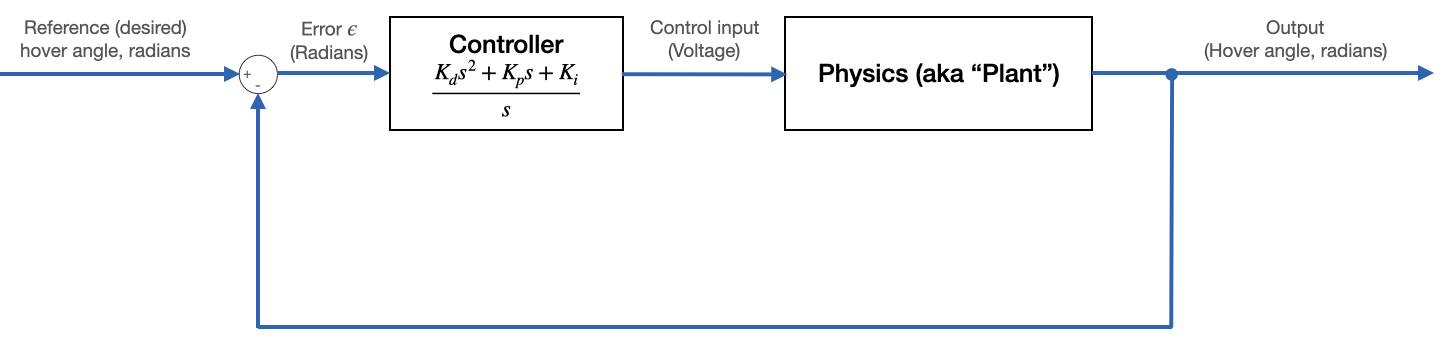
Building a PID controller
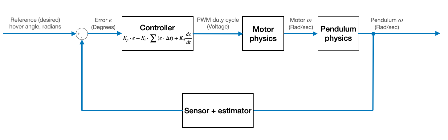
We are going to add a controller of the form shown below, where $K_d$ is the derivative gain, $K_p$ is the proportional gain, and $K_i$ is the integral gain. The plant physics is given by the transfer function above. The objective is to increase its speed (increase the magnitude of the output) without destabilizing it.
Note that the specific values for the gains will not be the same as in lab. The objective here is to see how the open-loop Bode plot changes as we add proportional, integral, and derivative terms to our PID controller.
Proportional term
Let us start by adding proportional gain. This has the effect of lifting the magnitude plot to greater values without affecting the phase plot. This decreases (but does not eliminate) steady state error and increases the system response speed. But! It also decreases our gain margin! Note that the gain margin decreases as the magnitude plot increases, and eventually the system goes unstable (has a gain of 0dB at 180 degrees of phase). This results in the persistent oscillations shown below.
The Bode plot for the proportionally-compensated ($K_p=7000$) system below is stable, but barely. How far above -180 degrees is the phase plot when the gain crosses 0dB? How far below 0dB is the gain plot when the phase crosses -180? We get significant oscillation, as shown in the video.
This is the Bode plot for the open-loop system. But the step response is for the closed-loop system. Recall that, for unity gain feedback, the closed loop transfer function is given by:
\begin{align} H(s) &= \frac{G(s)}{1+G(s)} \end{align}So, in this case, the closed-loop transfer function is:
\begin{align} H(s) &= \frac{K_p \alpha}{\beta s^4 + \gamma s^3 + \epsilon s^2 + \lambda s + \mu + K_p \alpha} \end{align}Kp = 7000
sys4 = signal.TransferFunction([Kp*alpha],
[beta, gamma, epsilon, lambdas, mu+(Kp*alpha)])
w, mag, phase = signal.bode(sys4)
plt.figure()
plt.title('Bode plot for open-loop, proportionally-compensated system')
plt.grid('on')
plt.semilogx(w, mag) # Bode magnitude plot
plt.ylabel('dB')
plt.figure()
plt.semilogx(w, phase) # Bode phase plot
plt.grid('on')
plt.xlabel('Rad/sec')
plt.ylabel('Degrees')
plt.show()


Step response, look at all that bouncing! We're approaching marginal stability.
Kp = 7000

lti = signal.lti(  [Kp*alpha],
                    [beta, gamma, epsilon, lambdas, mu+(Kp*alpha)])
t, y = signal.step2(lti, T=numpy.linspace(0, 10, 1000))
plt.title('Step response of pendulum with proportional control');plt.plot(t,y)
plt.grid('on')
plt.xlabel('sec'); plt.ylabel('Rad/sec');plt.show()

What would happen if we increased $K_p$ too much? Our phase margin would eventually become negative, and we go unstable! We can see that in the plot below, which uses $K_p = 8000$, making the system unstable.
Kp = 8000

lti = signal.lti(  [Kp*alpha],
                    [beta, gamma, epsilon, lambdas, mu+(2*Kp*alpha)])
t, y = signal.step2(lti, T=numpy.linspace(0, 10, 1000))
plt.title('Step response of pendulum with too-high proportional control');plt.plot(t,y)
plt.grid('on')
plt.xlabel('sec'); plt.ylabel('Rad/sec');plt.show()

Derivative term
We can stabilize the system by adding a derivative term to the controller. The derivative term will add phase, improving our gain and phase margins and thus improving stability (at the cost of system speed). The first Bode plot below shows the gain/phase of the PD controller, and the second shows the controller+physics open-loop system. Note that we begin adding phase at approximately the resonant frequency of the pendulum. See the Bode plot below, and notice that the gain and phase margins are much improved.
Kp = 55000
Kd = 5000.
Ki = 0

sys7 = signal.TransferFunction([Kd, Kp, Ki],
                               [ 1, 0])
w, mag, phase = signal.bode(sys7)

plt.figure()
plt.title('Bode plot for PD controller')
plt.grid('on')
plt.semilogx(w, mag)    # Bode magnitude plot
plt.ylabel('dB')
plt.figure()
plt.semilogx(w, phase)  # Bode phase plot
plt.grid('on')
plt.xlabel('Rad/sec')
plt.ylabel('Degrees')
plt.show()


Kp = 55000
Kd = 5000
Ki = 0

sys5 = signal.TransferFunction([Kd*alpha, Kp*alpha, 0],
                                [beta, gamma, epsilon, lambdas+(Kd*alpha), mu + (Kp*alpha), 0])
w, mag, phase = signal.bode(sys5)

plt.figure()
plt.title('Bode plot for open-loop, PD-compensated system')
plt.grid('on')
plt.semilogx(w, mag)    # Bode magnitude plot
plt.ylabel('dB')
plt.figure()
plt.semilogx(w, phase)  # Bode phase plot
plt.grid('on')
plt.xlabel('Rad/sec')
plt.ylabel('Degrees')
plt.show()


What's our closed-loop step response look like now? We have much less ringing! I've also increased $K_p$, so we have some overshoot, but the oscillations get damped out. Our closed-loop PD-compensated transfer function is:
\begin{align} H(s) &= \frac{K_d \alpha s + K_p \alpha}{\beta s^5 + \gamma s^4 + \epsilon s^3 + (\lambda + K_d \alpha) s^2 + (\mu + K_p \alpha) s} \end{align}Kp = 65000
Kd = 5000
Ki = 0
lti = signal.lti([Kd*alpha, Kp*alpha, 0],
[beta, gamma, epsilon, lambdas+(Kd*alpha), mu + (Kp*alpha), 0])
t, y = signal.step2(lti, T=numpy.linspace(0, 10, 1000))
plt.title('Step response of pendulum with PD control');plt.plot(t,y)
plt.grid('on')
plt.xlabel('sec'); plt.ylabel('Rad/sec');plt.show()

If our $K_d$ were smaller, we'd see more overshoot and less damping:
Kp = 65000
Kd = 2000
Ki = 0

lti = signal.lti([Kd*alpha, Kp*alpha, 0],
                 [beta, gamma, epsilon, lambdas+(Kd*alpha), mu + (Kp*alpha), 0])
t, y = signal.step2(lti, T=numpy.linspace(0, 10, 1000))
plt.title('Step response of pendulum with PD control, lower $K_d$');plt.plot(t,y)
plt.grid('on')
plt.xlabel('sec'); plt.ylabel('Rad/sec');plt.show()

Integral term
Finally, we must increase the system type (the number of free integrators in the open-loop transfer function) by 1 in order to eliminate steady-state error. We do this by adding an integral term to the controller. The relative magnitude of this term will be quite small because the integral term will remove phase and thus destabilize our system. This is a small term that, over time, will creep up on the target step input.
The first Bode is that of the PID controller, the second is that of the open-loop controller+physics.
In the video below, note that the integral term very slowly creeps the arm to the target hover angle.
Kp = 55000
Kd = 5000
Ki = 20000

sys8 = signal.TransferFunction([Kd, Kp, Ki],
                               [ 1, 0])
w, mag, phase = signal.bode(sys8)

plt.figure()
plt.title('Bode plot for PID controller')
plt.grid('on')
plt.semilogx(w, mag)    # Bode magnitude plot
plt.ylabel('dB')
plt.figure()
plt.semilogx(w, phase)  # Bode phase plot
plt.grid('on')
plt.xlabel('Rad/sec')
plt.ylabel('Degrees')
plt.show()


Here is the Bode-plot for the open-loop, PID compensated system:
Kp = 55000
Kd = 5000
Ki = 20000

sys6 = signal.TransferFunction(  [Kd*alpha, Kp*alpha, Ki*alpha],
                                 [beta, gamma, epsilon, lambdas+(Kd*alpha), mu + (Kp*alpha), Ki*alpha])
w, mag, phase = signal.bode(sys6)

plt.figure()
plt.title('Bode plot for open-loop, PID-compensated system')
plt.grid('on')
plt.semilogx(w, mag)    # Bode magnitude plot
plt.ylabel('dB')
plt.figure()
plt.semilogx(w, phase)  # Bode phase plot
plt.grid('on')
plt.xlabel('Rad/sec')
plt.ylabel('Degrees')
plt.show()


And the step response for that closed-loop system. The closed-loop transfer function for the PID-compensated system is given by:
\begin{align} H(s) &= \frac{K_d \alpha s + K_p \alpha + K_i \alpha}{\beta s^5 + \gamma s^4 + \epsilon s^3 + (\lambda + K_d \alpha) s^2 + (\mu + K_p \alpha) s + K_i \alpha} \end{align}Note how the steady-state error is eliminated!
Kp = 55000
Kd = 5000
Ki = 20000

lti = signal.lti([Kd*alpha, Kp*alpha, Ki*alpha],
                                 [beta, gamma, epsilon, lambdas+(Kd*alpha), mu + (Kp*alpha), Ki*alpha])
t, y = signal.step2(lti, T=numpy.linspace(0, 10, 1000))
plt.title('Step response of pendulum');plt.plot(t,y)
plt.grid('on')
plt.xlabel('sec'); plt.ylabel('Rad/sec');plt.show()
