HTML('''<script>code_show=true; function code_toggle() { if (code_show){ $('div.input').hide(); } else { $('div.input').show(); } code_show = !code_show} $( document ).ready(code_toggle);</script><form action="javascript:code_toggle()"><input type="submit" value="Click here to toggle on/off the raw code."></form>''')
In this lab, you are challenged to use the hardware resources on the FPGA as wisely as you can to accelerate a simulation of the 2D wave equation on a square mesh. The amplitude of the center node in the mesh will be communicated to the DAC at 48kHz to produce drum-like sounds. Your simulation will include a nonlinear effect related to the instantaneous tension in the mesh that produces the pitch-glide heard in real drums.
You are challenged to simulate the largest drum that you can. The group that uses the DSP blocks and memory blocks on the FPGA most exhaustively (as few as possible left over) and efficiently (as many as possible being used in parallel) will be able to produce the largest drum. Last year, the winning group's drum contained over 88,000 nodes!
You will be asked to compare the sizes of the largest drums that you can simulate using only the HPS vs. the FPGA. This lab will give you a sense of the FPGA's power for hardware acceleration.
A wave equation relates time derivatives to spatial derivates. The continuous form of the 2D wave equation is given below, where $c$ is the speed of sound and $u$ is the out-of-plane amplitude of the node.
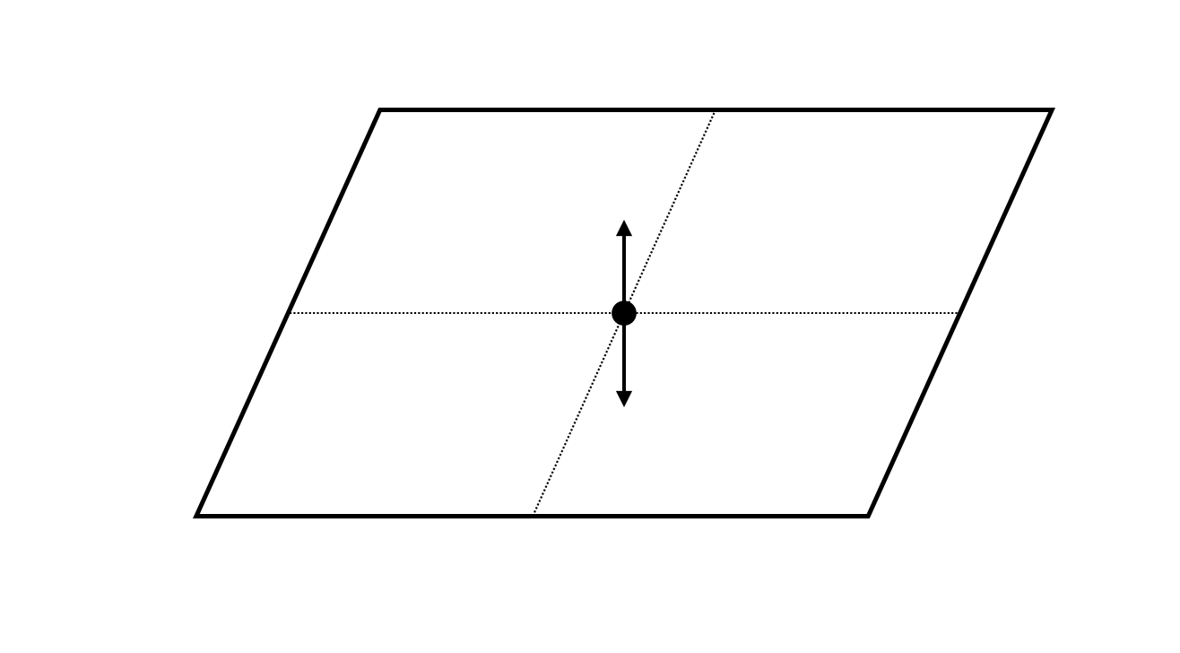
In order to implement this equation on the FPGA, we will used the discretized version shown below. For a derivation of the below equation from the above equation, see this webpage. The amplitude of a particular node, $u_{i,j}$ at the next timestep, $n+1$, is a function of the node's amplitude at the current and previous timesteps ($n$ and $n-1$) and the amplitudes of the four adjacent nodes at the current timestep.
(Take a close look at that first term. If $\frac{\eta \Delta t}{2}$ is small, is there an opportunity for simplification?) All of the other terms in the above expression are constants, except for $\rho_{eff}$. The value for this term is nonlinearly related to the amplitude of the center node according to the equation given below. This nonlinear coupling generates an audible "pitch-glide" just like is heard in real drums. In order for the drum to be stable, this value must be less than 0.5.
Matlab program from Bruce gives a sequential version of the algorithm and plots the Fourier modes of the drum.
Clicking "show code" at the top of this webpage will reveal Python code by Hunter based on Bruce's Matlab code (for the more Pythonically inclined person). Like the Matlab, it gives a sequential version of the algorithm and plots the Fourier modes of the drum. Plots given below. It compares the simulated and theoretical drum modes, as given in Physical Modeling with the 2-D Digital Waveguide Mesh.
Bruce's HPS code which implements the above equation in C for realtime synthesis on the HPS
If you play with the boundary conditions, damping, wave speed, drum size, and initial conditions, the sound will be drum-like, chime-like, gong-like, or bell-like.
In [1320]:
# Initializize drumn=100;u=numpy.zeros((n,n));u1=numpy.zeros((n,n));u2=numpy.zeros((n,n));uHit=numpy.zeros((n,n));# Set rho, sample rate, and simulation timerho=0.25;Fs=48000;time=numpy.arange(0,1.,(1./Fs))# Array in which to store audio samplesaud=numpy.zeros(len(time));# Compute middle nodesx_mid=int(n/2.);y_mid=int(n/2.);# Initialize drum amplitudes to a pyramidforiinrange(1,n-1):forjinrange(1,n-1):uHit[i,j]=max(0,30-(abs(x_mid-i)+abs(y_mid-j)))/30.;# Zero boundary conditionsuHit[0,:]=0uHit[n-1,:]=0uHit[:,0]=0uHit[:,n-1]=0# Indexing variabletindex=0;# Loop through time arrayfortintime:u=numpy.zeros((n,n))# Hit the drum at t=0if(t==0):u1=u1+uHit;# Compute updated drum amplitudesu[1:n-2,1:n-2]=(1./(1+.0001))*(rho*(u1[2:n-1,1:n-2]+u1[0:n-3,1:n-2]+u1[1:n-2,2:n-1]+u1[1:n-2,0:n-3]-4*u1[1:n-2,1:n-2])+2*u1[1:n-2,1:n-2]-(1-.0001)*(u2[1:n-2,1:n-2]));# Amplitude of center node goes into audio arrayaud[tindex]=u[n//2,n//2];# Update/store drum stateu2=u1;u1=u;# Iteratetindex=tindex+1;# Plot the center node amplitudesplt.plot(time,aud)plt.xlabel('time (sec)')plt.ylabel('amplitude')plt.title('Center-Node Amplitude and Power Spectrum for 100x100 drum',fontsize=18)plt.figsize=(20,3)plt.show()# Plot the power spectrumplt.rcParams["figure.figsize"]=(20,3)Pxxt,freqst=plt.psd(aud,NFFT=len(aud),Fs=48000,window=numpy.hamming(len(aud)),noverlap=50,label='100x100')# Plot the theoretical mode locationsfundamental=173yvals=numpy.linspace(-60,70)modes=[1.58,2.0,2.24,2.55,2.92,3.0,3.16,3.54]plt.plot(numpy.ones(len(yvals))*fundamental,yvals,'red',alpha=0.5,label='theoretical mode locations')foriinmodes:plt.plot(numpy.ones(len(yvals))*fundamental*i,yvals,'red',alpha=0.5)# Configure plotsplt.xlim([0,1000])plt.xticks(size=18)plt.legend(loc='best')plt.show()# Output audioprint("Audio - Python synthesized, 100x100 drum")Audio(aud,rate=48000)
Audio - Python synthesized, 100x100 drum
Out[1320]:
In [1317]:
# Initializize drumn=100;u=numpy.zeros((n,n));u1=numpy.zeros((n,n));u2=numpy.zeros((n,n));uHit=numpy.zeros((n,n));# Set rho, sample rate, and simulation timerho=0.25;rho_eff=0.25;Fs=48000;time=numpy.arange(0,1,(1./Fs))# Array in which to store audio samplesaud=numpy.zeros(len(time));# Compute middle nodesx_mid=int(n/2.);y_mid=int(n/2.);# Initialize drum amplitudes to a pyramidforiinrange(1,n-1):forjinrange(1,n-1):uHit[i,j]=max(0,30-(abs(x_mid-i)+abs(y_mid-j)))/30.;# Zero boundary conditionsuHit[0,:]=0uHit[n-1,:]=0uHit[:,0]=0uHit[:,n-1]=0# Indexing variabletindex=0;# Loop through time arrayfortintime:u=numpy.zeros((n,n))# Hit the drum at t=0if(t==0):u1=u1+uHit;# Compute updated drum amplitudesu[1:n-2,1:n-2]=(1./(1+.0001))*(rho_eff*(u1[2:n-1,1:n-2]+u1[0:n-3,1:n-2]+u1[1:n-2,2:n-1]+u1[1:n-2,0:n-3]-4*u1[1:n-2,1:n-2])+2*u1[1:n-2,1:n-2]-(1-.0001)*(u2[1:n-2,1:n-2]));# Amplitude of center node goes into audio arrayaud[tindex]=u[n//2,n//2];# Update/store drum stateu2=u1;u1=u;# Update rhorho_eff=min(0.49,rho+((1./16)*u[n//2,n//2])**2.)# Iteratetindex=tindex+1;# Output audioprint("Audio - Python synthesized, nonlinear (exaggerated) rho, 100x100 drum")Audio(aud,rate=48000)
Get the linear 2D PDE drum synthesis HPS code running (available on the DSP page, and also linked here
The above HPS code will help you write your Verilog.
Modify the code for athe nonlinear rho effect
Scale up the HPS solution until it is no longer realtime
Use synthesizable Verilog running in ModelSim to simulate a single node with zero boundary conditions.
Single node, zero boundary conditions
The result should be simple harmonic motion
Remember that rho<0.5. Start with rho=1/16.
Note that when rho is close to the limit of 0.5, the solution has a very high natural frequency, so the sine wave will be on the border of aliasing and thus look like a square wave.
Assuming 1.17 fixed point, start with initial conditions $u^n = u^{n-1}$ and an amplitude of about 1/8 full scale
ModelSim output for a single node with zero boundary conditions
Use synthesizable Verilog running in ModelSim to simulate a single column of nodes of length ~30 and with zero boundary conditions on the edges and on either end. You may find these slides helpful.
Column of nodes
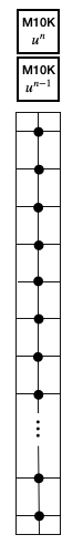
Store the initial amplitudes for the $n$ and $n-1$ timesteps in M10k memory blocks.
Create a state machine that reads a node amplitudes from M10k memory, computes their updated amplitudes, and writes those updated amplitudes back to M10k memory. The state machine will start at the bottom of the column and move to the top.
Remember that node updates must be synchronous. Otherwise your drum will be unconditionally unstable.
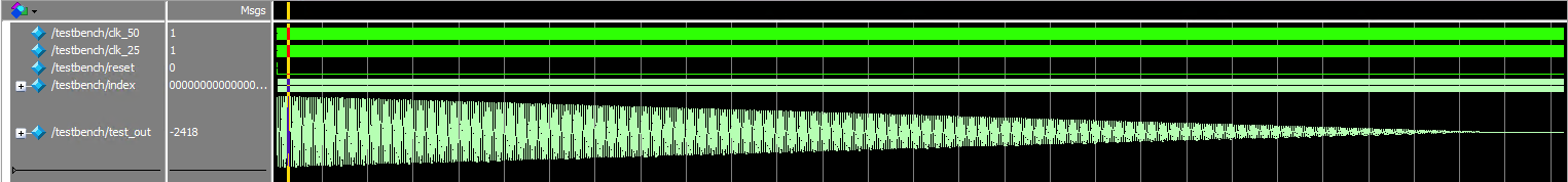
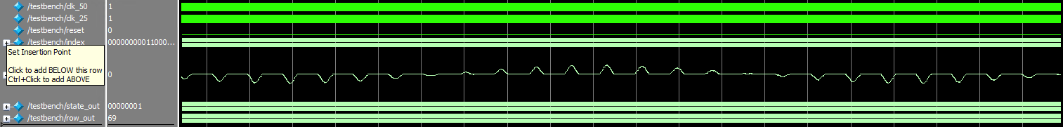
Initialize the node amplitudes in a triangle shape (highest in the middle, linearly falling to zero at the ends). View the node amplitudes in ModelSim. You should see the node amplitudes oscillate back and forth, with their amplitudes decaying over time.
Column of nodes oscillating
Column of nodes oscillating with decayed amplitude at later time
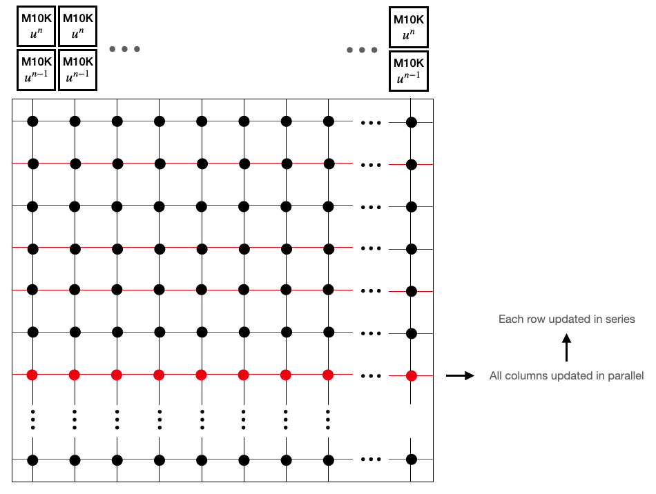
Using a generate statement, instantiate and connect 30 node columns. This will create a 30x30 drum for which all columns are update in parallel, and each row is updated in series.
30x30 drum. Columns updated in parallel, rows updated in series
Give all nodes reasonable initial conditions. Remember that you cannot just give the center node nonzero amplitude (spatial aliasing will occur). Your drum must be initialized with amplitudes that relatively smoothly transition from high in the center to zero at the boundaries. A pyramid works just fine.
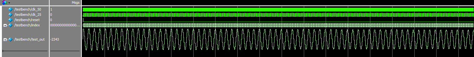
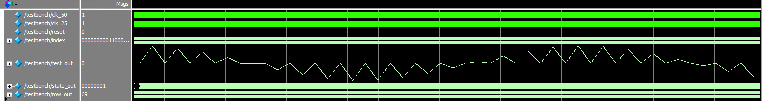
Output the amplitude of the center node in ModelSim. It will look something like that shown below.
Amplitude of center node for 30x30 drum
Export these data and play the sound that they generate with Matlab or Python. It should sound vaguely like a cowbell or a woodblock.
Add the nonlinear rho calculation to your ModelSim simulation.
Add synchronization signals to your ModelSim simulation.
Add computation time to your ModelSim simulation.
Download the Audio output bus_master example from the Quartus 18.1 page..
This example performs direct digital synthesis of a sine wave, with frequency controlled by the switches
Get it running and listen to it.
Integrate a drum of any size with this example (a column is fine, or a small square drum)
Integrate your drum synthesizer into the Audio output bus_master example from the Quartus 18.1 page.
Use hardcoded parameters
Use a 30x30 drum
Compile time will be approximately 9 minutes
Should sound like a cowbell or woodblock
Look at the compilation report to confirm that your multiplier usage is what you expect for it to be
With the 30-column drum, make the number of rows, the rho gain, and the initial amplitude of the drum configurable via PIO ports and/or the onboard switches and buttons.
Compile and test, compile time will be about 9 minutes
Scale up! Add as many columns to the drum as you can, making sure that you don't exceed 174 multipliers.
Your grid should have no more than 4:1 aspect ratio
Grid expansion via symmetry does not count for size
Compile time will be >20 minutes
Through your user interface (either PIO or switches) increase the number of rows in the drum until you can no longer meet timing requirements.
Listen to the drum with headphones that have nice bass, or through a subwoofer
Look for opportunities to optimize (pipeline your drum simulator? add a faster PLL to achieve more rows?)
In your demonstration, you will be asked to
Demonstrate the largest drum that you can simulate in realtime (no more than 4:1 aspect ratio)
Demonstrate at least three different drum sounds
At least one sound must include audible nonlinear tension modulation effects
Prove that the computation finishes in less than 20.8 $\mu s$ for your drums
Mathematical considerations (what you actually implemented)
A table of grid size vs. compute time for both the FPGA solver and the HPS solver
Do you see any cache-size effects on HPS? What is the effect of -O0 vs. -O3?
Are there any scaling surprises in the FPGA?
A description of your parallelization scheme
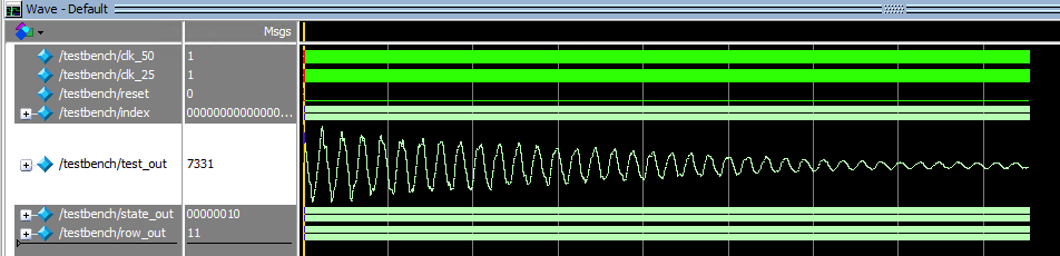
A plot of the power spectrum of your drum sounds for a few different drum sizes (example shown below)
For the largest square drum that you can synthesize, compare the theoretical frequencies for the drum modes to the modes visible on your power spectrum (see below)
A screenshot from the chip planner for your biggest drum, showing hardware utilization
A heavily commented listing of your Verilog and GCC code.